- •Preface
- •Contents
- •1 Introduction
- •1.1 Physics
- •1.2 Mechanics
- •1.3 Integrating Numerical Methods
- •1.4 Problems and Exercises
- •1.5 How to Learn Physics
- •1.5.1 Advice for How to Succeed
- •1.6 How to Use This Book
- •2 Getting Started with Programming
- •2.1 A Python Calculator
- •2.2 Scripts and Functions
- •2.3 Plotting Data-Sets
- •2.4 Plotting a Function
- •2.5 Random Numbers
- •2.6 Conditions
- •2.7 Reading Real Data
- •2.7.1 Example: Plot of Function and Derivative
- •3 Units and Measurement
- •3.1 Standardized Units
- •3.2 Changing Units
- •3.4 Numerical Representation
- •4 Motion in One Dimension
- •4.1 Description of Motion
- •4.1.1 Example: Motion of a Falling Tennis Ball
- •4.2 Calculation of Motion
- •4.2.1 Example: Modeling the Motion of a Falling Tennis Ball
- •5 Forces in One Dimension
- •5.1 What Is a Force?
- •5.2 Identifying Forces
- •5.3.1 Example: Acceleration and Forces on a Lunar Lander
- •5.4 Force Models
- •5.5 Force Model: Gravitational Force
- •5.6 Force Model: Viscous Force
- •5.6.1 Example: Falling Raindrops
- •5.7 Force Model: Spring Force
- •5.7.1 Example: Motion of a Hanging Block
- •5.9.1 Example: Weight in an Elevator
- •6 Motion in Two and Three Dimensions
- •6.1 Vectors
- •6.2 Description of Motion
- •6.2.1 Example: Mars Express
- •6.3 Calculation of Motion
- •6.3.1 Example: Feather in the Wind
- •6.4 Frames of Reference
- •6.4.1 Example: Motion of a Boat on a Flowing River
- •7 Forces in Two and Three Dimensions
- •7.1 Identifying Forces
- •7.3.1 Example: Motion of a Ball with Gravity
- •7.4.1 Example: Path Through a Tornado
- •7.5.1 Example: Motion of a Bouncing Ball with Air Resistance
- •7.6.1 Example: Comet Trajectory
- •8 Constrained Motion
- •8.1 Linear Motion
- •8.2 Curved Motion
- •8.2.1 Example: Acceleration of a Matchbox Car
- •8.2.2 Example: Acceleration of a Rotating Rod
- •8.2.3 Example: Normal Acceleration in Circular Motion
- •9 Forces and Constrained Motion
- •9.1 Linear Constraints
- •9.1.1 Example: A Bead in the Wind
- •9.2.1 Example: Static Friction Forces
- •9.2.2 Example: Dynamic Friction of a Block Sliding up a Hill
- •9.2.3 Example: Oscillations During an Earthquake
- •9.3 Circular Motion
- •9.3.1 Example: A Car Driving Through a Curve
- •9.3.2 Example: Pendulum with Air Resistance
- •10 Work
- •10.1 Integration Methods
- •10.2 Work-Energy Theorem
- •10.3 Work Done by One-Dimensional Force Models
- •10.3.1 Example: Jumping from the Roof
- •10.3.2 Example: Stopping in a Cushion
- •10.4.1 Example: Work of Gravity
- •10.4.2 Example: Roller-Coaster Motion
- •10.4.3 Example: Work on a Block Sliding Down a Plane
- •10.5 Power
- •10.5.1 Example: Power Exerted When Climbing the Stairs
- •10.5.2 Example: Power of Small Bacterium
- •11 Energy
- •11.1 Motivating Examples
- •11.2 Potential Energy in One Dimension
- •11.2.1 Example: Falling Faster
- •11.2.2 Example: Roller-Coaster Motion
- •11.2.3 Example: Pendulum
- •11.2.4 Example: Spring Cannon
- •11.3 Energy Diagrams
- •11.3.1 Example: Energy Diagram for the Vertical Bow-Shot
- •11.3.2 Example: Atomic Motion Along a Surface
- •11.4 The Energy Principle
- •11.4.1 Example: Lift and Release
- •11.4.2 Example: Sliding Block
- •11.5 Potential Energy in Three Dimensions
- •11.5.1 Example: Constant Gravity in Three Dimensions
- •11.5.2 Example: Gravity in Three Dimensions
- •11.5.3 Example: Non-conservative Force Field
- •11.6 Energy Conservation as a Test of Numerical Solutions
- •12 Momentum, Impulse, and Collisions
- •12.2 Translational Momentum
- •12.3 Impulse and Change in Momentum
- •12.3.1 Example: Ball Colliding with Wall
- •12.3.2 Example: Hitting a Tennis Ball
- •12.4 Isolated Systems and Conservation of Momentum
- •12.5 Collisions
- •12.5.1 Example: Ballistic Pendulum
- •12.5.2 Example: Super-Ball
- •12.6 Modeling and Visualization of Collisions
- •12.7 Rocket Equation
- •12.7.1 Example: Adding Mass to a Railway Car
- •12.7.2 Example: Rocket with Diminishing Mass
- •13 Multiparticle Systems
- •13.1 Motion of a Multiparticle System
- •13.2 The Center of Mass
- •13.2.1 Example: Points on a Line
- •13.2.2 Example: Center of Mass of Object with Hole
- •13.2.3 Example: Center of Mass by Integration
- •13.2.4 Example: Center of Mass from Image Analysis
- •13.3.1 Example: Ballistic Motion with an Explosion
- •13.4 Motion in the Center of Mass System
- •13.5 Energy Partitioning
- •13.5.1 Example: Bouncing Dumbbell
- •13.6 Energy Principle for Multi-particle Systems
- •14 Rotational Motion
- •14.2 Angular Velocity
- •14.3 Angular Acceleration
- •14.3.1 Example: Oscillating Antenna
- •14.4 Comparing Linear and Rotational Motion
- •14.5 Solving for the Rotational Motion
- •14.5.1 Example: Revolutions of an Accelerating Disc
- •14.5.2 Example: Angular Velocities of Two Objects in Contact
- •14.6 Rotational Motion in Three Dimensions
- •14.6.1 Example: Velocity and Acceleration of a Conical Pendulum
- •15 Rotation of Rigid Bodies
- •15.1 Rigid Bodies
- •15.2 Kinetic Energy of a Rotating Rigid Body
- •15.3 Calculating the Moment of Inertia
- •15.3.1 Example: Moment of Inertia of Two-Particle System
- •15.3.2 Example: Moment of Inertia of a Plate
- •15.4 Conservation of Energy for Rigid Bodies
- •15.4.1 Example: Rotating Rod
- •15.5 Relating Rotational and Translational Motion
- •15.5.1 Example: Weight and Spinning Wheel
- •15.5.2 Example: Rolling Down a Hill
- •16 Dynamics of Rigid Bodies
- •16.2.1 Example: Torque and Vector Decomposition
- •16.2.2 Example: Pulling at a Wheel
- •16.2.3 Example: Blowing at a Pendulum
- •16.3 Rotational Motion Around a Moving Center of Mass
- •16.3.1 Example: Kicking a Ball
- •16.3.2 Example: Rolling down an Inclined Plane
- •16.3.3 Example: Bouncing Rod
- •16.4 Collisions and Conservation Laws
- •16.4.1 Example: Block on a Frictionless Table
- •16.4.2 Example: Changing Your Angular Velocity
- •16.4.3 Example: Conservation of Rotational Momentum
- •16.4.4 Example: Ballistic Pendulum
- •16.4.5 Example: Rotating Rod
- •16.5 General Rotational Motion
- •Index
12.3 Impulse and Change in Momentum |
363 |
||
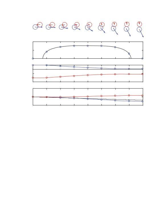
Fig. 12.6 Illustration of the |
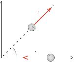
y |
||
velocity of a tennis ball |
|
|
|
before and after it was hit by |
|
|
1 |
|
v |
||
a racket |
|
|
|
|
v |
0 |
|
x |
We find the x - and y-components of the impulse:
Jx = J · i = m |
vx ,1 − vx ,0 |
|
= 57 g (15 cos α + 20) m/s = 1.74 kg m/s (12.37) |
Jy = J · j = m |
vx ,1 − vx ,0 |
|
= 57 g (15 sin α − 0) m/s = 0.60 kg m/s . (12.38) |
The impulse is therefore:
J = 1.74 kg m/s i + 0.60 kg m/s j , |
(12.39) |
The force is given as the impulse divided by the time interval. We assume the time interval to be the same for this process, t = 2 ms. The average net force is therefore:
J1.74 kg m/s i + 0.60 kg m/s j
Favg = |
|
= |
|
= 870 N i + 300 N j , (12.40) |
|
|
|||
|
t |
2 10−3 s |
Interestingly, this means that the direction of the net force is in the direction β:
β = tan |
−1 Fy |
◦ |
|
|
|
|
= 19 . |
(12.41) |
|
|
|
Fx
12.4 Isolated Systems and Conservation of Momentum
During a collision between two objects the forces acting between the objects generally have a complicated time dependence—the curve of F (t ) is non-trivial. It is therefore not a simple task to calculate the impulse integral and use this to determine the change in momentum of the objects. Fortunately, it turns out that the problem can be significantly simplified for an isolated system where the net external force is zero. In this case the total momentum of the system is conserved throughout the collision. The total momentum is therefore the same before and after the collision. This is a powerful principle we use to analyze complex interactions without determining the detailed motion and forces in the system.
364 |
12 Momentum, Impulse, and Collisions |
Momentum and Motion of Two Objects
We will now demonstrate that the total momentum is conserved when there are no external forces by discussing the collision between two objects A and B, illustrated in Fig. 12.7. We know that we can determine the motion of each object from Newton’s second law of motion applied to each of the objects. For each object we separate the forces into external forces, forces having an origin outside the system, and internal forces, forces that are acting between the two objects:
Internal forces act between the objects in the system.
External forces act between objects in the system and the environment.
For the collision in Fig. 12.7 the only internal forces are the forces between the objects: The force from A on B and the reaction force from B on A. With this notation, Newton’s second law for object A can be written as:
F A = FextA + FB on A = |
dpA |
, |
(12.42) |
dt |
where the sum is over all the external forces acting on object A. Similarly, Newton’s second law for object B is:
FB = FextB + F A on B = |
dpB |
, |
(12.43) |
dt |
where we again have summed over all the external forces acting on object B. Now, we do not want to address the internal forces acting between A and B. How can we
F [ N ]
4
2
0
0 |
0.005 |
0.01 |
0.015 |
0.02 |
0.025 |
0.03 |
0.035 |
0.04 |
t [ s]
Fig. 12.7 Illustration of a collision between two objects A (red) and B (blue). The top figure shows the forces FB on A (red) and F A on B (blue) acting between the objects at various times ti throughout the collision. The bottom figure shows the magnitude of the force, F (t ), as a function of time. The time ti that are shown in the top figure is illustrated by circles
12.4 Isolated Systems and Conservation of Momentum |
365 |
get rid of them in these equations? There is a commonly used trick: we recall from Newton’s thirds law that the reaction force F A on B is equal, but oppositely directed to FB on A :
F A on B = −FB on A , |
(12.44) |
If we insert this into (12.43), we get two equations for the motion of object A and B:
FextA |
+ FB on A = |
dpA |
|
dt |
|
||
FextB |
− FB on A = |
dpB |
(12.45) |
dt |
If we add the equations, we get rid of the internal forces, FB on A :
FextA + FextB = |
dpA |
+ |
dpB |
, |
(12.46) |
dt |
dt |
We introduce the sum over all the external forces on all the objects in the system: Over all the forces acting on object A and all the forces acting on object B:
Fext = FextA + FextB . |
(12.47) |
|||
We use this to simplify (12.46): |
|
|
|
|
Fext |
|
d |
|
|
= |
|
(pA + pB ) . |
(12.48) |
|
dt |
We call the sum of the momenta for each of the objects the total momentum of the system:
Total momentum: |
p = pA + pB , |
|
P = |
(12.49) |
This provides a generalization of Newton’s second law for a two-particle-system:
Generalization of Newton’s second law:
Fext |
|
d |
p = |
d |
|
|
= |
|
|
(pA + pB ) , |
(12.50) |
||
dt |
dt |
366 |
12 Momentum, Impulse, and Collisions |
This law is completely general. We have not made any assumptions about the interactions between the two objects. The internal and external forces may be of any kind, conservative or non-conservative. The law is valid in all cases.
Conservation of Momentum in Isolated Systems
As a special case of this law, we observe that if the net external force on the system is zero (or negligible), the total momentum of the system is conserved:
Fext |
d |
|
= 0 dt (pA + pB ) = 0 . |
(12.51) |
We call a system isolated if the net external force is zero (or negligible):
An isolated system is a collection of objects that may interact internally, but
where the net external force on all the objects is zero (or negligible).
For an isolated system, the total momentum is conserved:
pA + pB = constant (for an isolated system) . |
(12.52) |
•This is a completely general law for the conservation of momentum of a system. It only requires the net external force on the system to be zero. It is valid not only at the beginning and at the end of the collision, but at all times during the collision as well.
•Notice: A common mistake is to forget the absolutely necessary condition that the net external force on the system must be zero (or negligible). Whenever you employ this law, you should make a habit of always asking yourself if the net external force is zero, or if it is reasonable to neglect it compared with other forces.
•Notice that the conservation law is a vector equation, and that it can be valid in one direction independently of an orthogonal direction. If the net external force in the x -direction is zero, the total momentum in this direction is conserved even though there is a net external force in the y-direction.
•Notice that it is not only valid for contact forces, as illustrated in Fig. 12.7, but for any type of force, including long-reaching forces such as gravity. The gravitational forces between object in the system are internal forces, while gravitational forces between objects in the system and objects outside the system are external forces.
12.4 Isolated Systems and Conservation of Momentum |
367 |
p [ kg m / s] p [ kg m / s] Y X
4
[N ] |
|
|
|
|
|
|
|
|
2 |
|
|
|
|
|
|
|
|
F |
|
|
|
|
|
|
|
|
0 |
|
|
|
|
|
|
|
|
0.1 |
|
|
|
|
|
|
|
|
0 |
|
|
|
|
|
|
|
|
−0.1 |
|
|
|
|
|
|
|
|
0.1 |
|
|
|
|
|
|
|
|
0 |
|
|
|
|
|
|
|
|
−0.1 |
|
|
|
|
|
|
|
|
0 |
0.005 |
0.01 |
0.015 |
0.02 |
0.025 |
0.03 |
0.035 |
0.04 |
t [ s]
Fig. 12.8 Illustration of the same process as in Fig. 12.7, but now the arrows in the top figure illustrates the momentum of the object, and the two bottom figures show the momentum px (t ) and py (t ) as a function of time. The total momentum is shown with a dotted line
Conservation of Total Momentum During a Collision
The conservation of total momentum during the collision between objects A and B is illustrated in Fig. 12.8. The arrows indicate the momentum of each object and the plots show the momentum in the x - and y-direction for each object and the total momentum. Since there are only internal forces acting in this system, there are no external forces affecting either object, and the total momentum is conserved in both the x - and the y-direction.
Conservation of Total Momentum During a Collision with an External Force
What happens if we addressed the same collision, but also include a gravitational force in the y-direction for both objects? As illustrated in Fig. 12.9, the behavior looks similar: The force as a function of time, F (t ), is similar, and the total momentum in the x -direction is conserved. However, the momentum in the y-direction is not conserved. It is decreasing throughout the motion due to the external force, gravity, acting on both object A and object B.
368 |
12 Momentum, Impulse, and Collisions |
p [ kg m / s] p [ kg m / s] Y X
4
[N ] |
|
|
|
|
|
|
|
|
2 |
|
|
|
|
|
|
|
|
F |
|
|
|
|
|
|
|
|
0 |
|
|
|
|
|
|
|
|
0.1 |
|
|
|
|
|
|
|
|
0 |
|
|
|
|
|
|
|
|
−0.1 |
|
|
|
|
|
|
|
|
0.2 |
|
|
|
|
|
|
|
|
0 |
|
|
|
|
|
|
|
|
−0.2 |
|
|
|
|
|
|
|
|
0 |
0.005 |
0.01 |
0.015 |
0.02 |
0.025 |
0.03 |
0.035 |
0.04 |
t [ s]
Fig. 12.9 Illustration of the same objects as in Figs. 12.7 and 12.8., but now with gravity acting in the y-direction. The arrows in the top figure illustrates the momentum of the objects. The bottom figures show the momentum px (t ) and py (t ) as a function of time. The total momentum (dotted line) is constant in the x -direction, but is changing in the y-direction due to the net force from gravity affecting the objects
How large is the effect of an external force, like gravity in this case? The change in momentum is given by the impulse of the external forces:
t1
P = Jext = |
Fextdt , |
(12.53) |
t0
To determine the effect of the external forces, we therefore need to compare the change of momentum due to the external force, P, to the total momentum of the system, P. For the gravitational force G = −mgæ, the impulse of gravity is:
t1 |
(12.54) |
JG,y = (−m A g − m B g) dt = − (m A + m B ) t , |
|
t0 |
|
and the total momentum in the y-direction of the whole system, |
|
Py = pA,y + pB,y = m A vA,0,y + m B vB,0,y . |
(12.55) |