


64 |
4 Motion in One Dimension |
gives significantly better solutions for many problems. This improved method is called Euler-Cromer’s method, and you can use this method safely for most problems you encounter.
In Euler-Cromer’s method to solve the (second order) differential equation of motion:
dt 2 |
= a t , x , |
dt |
, v(t0) = v0 , x (t0) = x0 , |
(4.51) |
d2 x |
|
d x |
|
|
we perform the following steps:
v(ti + |
t ) v(ti ) + a(ti , x (ti ), v(ti )) t |
|
x (ti + |
t ) x (ti ) + v(ti + t ) t |
(4.52) |
4.2.1 Example: Modeling the Motion of a Falling Tennis Ball
This example demonstrates how we can calculate the motion of a falling tennis ball given an expression for the acceleration.
Background: In Sect. 4.1.1 we studied the motion of a falling tennis ball based on measurements of its motion. However, in physics we do not only want to observe motion, we want to predict it. We do this by first analyzing the problem to find the forces acting on the object, and from the forces we find a mathematical model of the acceleration of the object. (You will learn to do this in the next chapter. For now we will assume that the acceleration is given). From the acceleration, we find the position and velocity by analytical or numerical integration. We call this recipe the structured problem-solving approach.
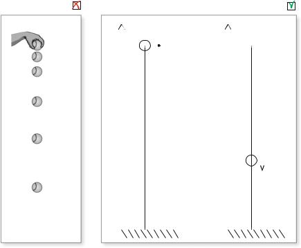
System sketch: Your first step should always be to make a sketch the process. In physics, our sketches are vessels for our thoughts. A good, functional sketch is therefore an important part of solving a problem. While the left part of Fig. 4.9 has a nice artistic appeal and also illustrates the motion in detail, we do not encourage such detailed sketches. Instead, you should make a sketch that only focuses on the most important features of the process, as in the rightmost figure. Here we illustrate the object (the tennis ball), its surroundings (most importantly the floor), and the coordinate system with a clearly marked axis. We have also illustrated the initial position and velocity of the ball, and its position and velocity at a time t . Drawing a simplified illustration helps you discern the important from the unimportant, and it helps you convert a physical situation into a mathematical problem: The figure shows the axis and the position of the ball, y(t ), and nothing else.
4.2 Calculation of Motion |
|
|
|
|
|
65 |
||||||
|
TOO DETAILED |
|
|
|
|
|
|
|
GOOD |
|||
|
|
|
|
y |
|
|
|
y |
|
|
|
|
|
|
|
|
|
|
|
|
|
|
|
||
|
0.0S |
y0 |
|
v0=0 |
y0 |
|
|
|
|
|||
|
|
|
|
|
|
|||||||
|
0.1S |
|
|
|
|
|
|
|
|
|
||
|
0.2S |
|
|
|
|
|
|
|
|
|
||
|
0.3S |
|
|
|
|
|
|
|
|
|
||
|
0.4S |
|
|
|
|
|
|
|
|
|
||
|
|
|
|
|
|
|
|
y(t) |
|
|
v(t) |
|
|
|
|
|
|
|
|
|
|
|
|||
|
|
|
|
|
|
|
|
|
|
|
||
|
0.5S |
|
|
|
|
|
|
|
|
|
||
|
|
|
|
|
|
|
|
|
|
|
||
|
30CM |
|
|
|
|
|
|
|
|
|
|
|
|
|
|
|
|
|
|
|
|
|
|
|
|
|
|
|
|
|
|
|
|
|
|
|
|
|
Fig. 4.9 Left Too detailed illustration. (Right) Correct, simple sketch
Simplified model: From an analysis of the physics of the system, we have found that the acceleration of the ball is a constant:
a = −g = −9.8 m/s2 . |
(4.53) |
(You will learn where this model comes from later. Now we only want to address the consequences of such a model). In addition, we know that the ball starts from rest at the position y0 = 2.0 m at the time t0 = 0 s:
y(0 s) = 2.0 m , v(0 s) = 0 m/s . |
(4.54) |
We have now formulated a mathematical description of the problem we want to solve:
|
dv |
= |
d2 y |
|
|
a = |
|
|
= −g , v(0) = v0 , y(0) = y0 . |
(4.55) |
|
dt |
dt 2 |
||||
Solving this equation means to find the velocity v(t ) and the position y(t ) of the ball for any time t . We call this the modeling step, finding the mathematical problem to solve, and the next step is to solve this problem—to find v(t ) and y(t ).

66 |
4 Motion in One Dimension |
Solving the simplified model: Since the acceleration is given and a constant, we can find the velocity by direct integration of the acceleration:
|
|
|
dv |
|
|
|
||
|
|
|
|
|
= −g; |
|
(4.56) |
|
t0 |
|
|
|
dt |
|
|||
|
dt |
|
dt = t0 |
−g dt , |
(4.57) |
|||
t dv |
|
|
t |
|
|
|
||
|
|
|
= −g t + g |
|
|
|||
v(t ) − v(t0) |
t0 , |
(4.58) |
||||||
|
|
|
|
|
|
|||
|
=0 m/s |
|
|
=0 s |
|
|||
which gives |
|
v(t ) = −gt . |
|
|
||||
|
|
|
(4.59) |
|||||
Similarly, we find the position by integrating the velocity:
|
d y |
= v(t ) , |
|
|
(4.60) |
||||||
|
|
|
|
|
|
||||||
0 |
|
|
dt |
|
|
||||||
dt |
dt = 0 |
v(t ) dt , |
(4.61) |
||||||||
t |
d y |
|
|
t |
|
|
|
|
|
|
|
y(t ) − y(0) = 0 |
−gt dt = − |
2 gt 2 , |
(4.62) |
||||||||
|
|
|
|
|
t |
|
|
|
1 |
|
|
which gives |
|
|
|
|
|
|
|
|
|
|
|
y(t ) = y(0) − |
1 |
gt 2 . |
|
|
(4.63) |
||||||
|
|
|
|
||||||||
|
2 |
|
|
||||||||
Analysis of the simplified model: This is the complete solution to the problem. We know the position and velocity as a function of time. When you have this solution, you are prepared to answer any question about the motion. For example, you can find out when the ball hits the ground and you can find the velocity of the ball when it hits the ground. How would you do that? You need to translate the question into a mathematical problem. We do this by stating the condition “when the ball hits the ground” in mathematical terms: The ball hits the ground when its position is that of the ground, that is, when y(t ) = 0 m. (Notice, we have ignored the extent of the ball here). We can use our solution in (4.63) to find the corresponding time:
y(t ) = y(0) − |
1 |
gt 2 = 0 m t = |
2 y(0) |
(4.64) |
|
|
|
. |
|||
2 |
g |
||||
A more realistic model: Unfortunately, data for the motion of the tennis ball, shown in Fig. 4.6b, show that the ball does not have a constant acceleration. This is due to
4.2 Calculation of Motion |
67 |
air resistance—an effect not included in the simplified model. Fortunately, we have good models for air resistance. For a falling ball in air, a more realistic model that includes the effect of air resistance is:
a = −g − Dv|v| , |
(4.65) |
where v = v(t ) is the velocity of the ball, g = 9.8 m/s2 is the same constant as above, and the constant D depends on details of the ball. For a tennis ball D = 0.0245 m−1 is a reasonable value. (You will learn about the background for this model and how to determine values for D later). We can now formulate a mathematical problem:
dv |
|
||
a = |
|
= −g − Dv|v| , |
(4.66) |
|
|||
|
dt |
|
|
with initial conditions v(0 s) = 0 m/s and y(0 s) = 2.0 m.
Solution of the realistic model: Our task is to solve this problem, which means to find v(t ) and y(t ) for the ball. This can be done either numerically or analytically. The numerical solution is straightforward, using the approach we have derived, but the analytical solution requires some knowledge of differential equations.
Numerical solution: We apply Euler-Cromer’s method to find the positions and velocities by stepwise integration starting from the initial conditions. The integration step in Euler-Cromer’s method is:
v(ti + |
t ) = v(t0) + a(ti , vi , yi ) |
t |
(4.67) |
y(ti + |
t ) = y(t0) + v(ti + t ) |
t , |
(4.68) |
where we insert the acceleration from (4.65):
a(ti , vi , yi ) = −g − Dv(ti )|v(ti )| , |
(4.69) |
This is implemented as follows: We define the physical constants and values given in the problem: g, D, y(0) and v(0):
D = |
0.0245 |
# mˆ-1 |
|
g = |
9.8 |
# m/sˆ2 |
|
y0 |
= |
2.0 |
|
v0 |
= |
0.0 |
|
We need to determine for how long we want to calculate the motion: What will be our maximum value of t ? There are typically two strategies: We can make an initial guess for the duration of the simulation, or we can determine when the simulation should stop during the simulation. First, we make a guess for the duration of the simulation. Based on the existing data from Fig. 4.6 we guess that t = 0.5 s is a reasonable simulation time:
time = 0.5
68 4 Motion in One Dimension
Next, we need to decide the time-step t . This needs to be small enough to ensure a good precision of the result, but not too small or the simulation takes too long. We try a value of t = 0.00001 s:
dt = 0.00001
Based on this, we calculate how many simulation steps we need, n = t /Δt , and generate arrays for the positions, velocities, accelerations and time for the simulation. All values are initially set to zero:
# Variables
n = ceil(time/dt) y = zeros(n,float) v = zeros(n,float) a = zeros(n,float) t = zeros(n,float)
Then we set the initial conditions:
# Initialize y[0] = y0 v[0] = v0
Before, finally, the Euler-Cromer steps are implemented in an integration loop. The whole program is given in the following:
from pylab import * D = 0.0245 # mˆ-1
g = 9.8 |
# m/sˆ2 |
||
y0 |
= |
2.0 |
|
v0 |
= |
0.0 |
|
time = 0.5 dt = 0.00001
# Variables
n = ceil(time/dt) y = zeros(n,float) v = zeros(n,float) a = zeros(n,float) t = zeros(n,float)
#Initialize y[0] = y0 v[0] = v0
#Integration loop for i in range(n-1):
a[i] = -g -D*v[i]*abs(v[i]) v[i+1] = v[i] + a[i]*dt y[i+1] = y[i] + v[i+1]*dt t[i+1] = t[i] + dt
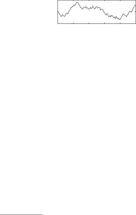
The resulting plots of x (t ), v(t ), and a(t ) are shown in Fig. 4.10.
Analysis of realistic model results: We can now use this result to answer questions like how long does it take until the ball hits the ground? Again, we answer the question by translating it into a mathematical question: The ball hits the ground when y(t ) = 0 m. However, in this case, we must find the solution numerically. The simplest approach to this would be to find when y becomes zero during the simulation. It is tempting to do this by checking when y(t ) = 0 m:
if (y[i]==0.0) print t[i]

4.2 Calculation of Motion
Fig. 4.10 Plots of y(t ), v(t ), and a(t ) calculated using the model for air resistance (black line) compared with analytical model (gray circles)
a [M/S2 ] v [M/S] y [M]
69
2 

1.5
1
0.50
t [S]
-2
-4
-9.2
t [S]
-9.4
-9.6
-9.8
0 |
0.1 |
0.2 |
0.3 |
0.4 |
0.5 |
t [S]
But this will not work, because y(ti ) will usually not be zero for any i . Typically, the program will step right past y = 0 going from a small positive value at some ti to a small negative value at ti +1. We should instead find the first time y(t ) passes 0, that is, we should find the first ti +1 when y(ti +1) < 0. Then we know that y(t ) = 0 somewhere in the interval ti < t < ti +1. We can then estimate a precise value for t using interpolation, or we can simply use the value ti +1, if we find that this gives us sufficient precision. This is implemented in the following modification to the program, where we have also stopped the calculation when the ball hits the ground:
for i in range(n-1):
a[i] = -g -D*v[i]*abs(v[i]) v[i+1] = v[i] + a[i]*dt y[i+1] = y[i] + v[i+1]*dt if (y[i+1]<0):
break
t[i+1] = t[i] + dt print v[i+1] plot(t[0:i-1],a[0:i-1]) xlabel(’t [s]’); ylabel(’a [m/sˆ2]’);
where we have used break to stop the loop when the condition is met. Notice that we should now only plot the values up to i, because we have not calculated any more values. The values from i + 2 to n were set to zero initially for y, v, and a and will make your plot confusing if you include them. (Try it and see).
Test your understanding: What would happen if we considered that the ball had an initial velocity v0 = −2vT when it started? Sketch the resulting position, velocity and acceleration as a function of time.
Analytical solution: The differential equation in (4.66) is one of a few equations we can solve analytically as long as the velocity does not change sign. When the ball is falling down, the velocity is negative, and we can replace |v| by −v:

70 |
|
4 Motion in One Dimension |
|
dv |
= −g − Dv (−v) = −g + D v2 . |
(4.70) |
|
|
|
||
|
dt |
||
This equation can be solved using separation of variables.
We separate the variables, so that all v’s are on the left side and all t ’s are on the right:
|
dv |
|
||
|
|
|
= −1 dt . |
(4.71) |
g |
− |
Dv2 |
||
|
|
|
|
|
The differential equation can now be solved by integrating each side from v0 = 0 m/s to v and from t0 = 0 s to t :
v0 g |
d Dv2 |
= |
t0 |
−1 dt = −t , |
(4.72) |
v |
v |
|
t |
|
|
−
The left-side integral can be solved using your knowledge from calculus (or by using the symbolic solver in Python) giving:
0 |
v |
g − Dv2 |
= g vT tanh−1 |
vT , |
(4.73) |
||||
|
|
dv |
1 |
|
|
|
|
v |
|
where we have introduced the quantity vT |
= √ |
|
to simplify the notation. We |
||||||
g/D |
|||||||||
notice that vT has dimensions m/s, and we may therefore call it a velocity. We insert (4.73) back into (4.72), getting
vT tanh−1 |
(v/vT ) |
= − |
gt |
|
v |
= |
vT tanh ( |
− |
gt /vT ) . |
(4.74) |
|
|
|
|
We have now found the velocity on the form v = v(t ), and we can simply integrate the velocity from t0 to t to find y(t ):
y(t ) − y(t0) = t0 |
v(t ) dt = 0 |
t |
vT tanh − vT dt . |
(4.75) |
|||
t |
|
|
|
|
gt |
|
|
This integral can solved by the symbolic integrator in Python giving: |
|
||||||
y(t ) = y(0) − v2T /g log cosh |
gt |
(4.76) |
|||||
|
. |
||||||
vT |
|||||||
Figure 4.10 shows that the analytical solutions (given by circles) are identical to the numerical solutions (lines).
Symbolic solution: The differential equation in (4.66) can also be solved directly using the symbolic solver in Python. We can solve the differential equation for the velocity, v(t ):
dv |
(4.77) |
= −g + D v2 , v(0) = 0 . |
dt
4.2 Calculation of Motion |
71 |
First, we define the variables g and D as symbolic variables, and the function v(t) as a symbolic functions:
>>from sympy import *
>>v = Function(’v’)
>>t = Symbol(’t’,real=True,positive=True)
>>g = Symbol(’g’,real=True,positive=True)
>>D = Symbol(’D’,real=True,positive=True)
Python can then solve the equation with the initial condition by
>> dsolve(Derivative(v(t),t)+g-D*v(t)**2,v(t)) -sqrt(1/(D*g))*log(-g*sqrt(1/(D*g)) + v(t))/2 +
... sqrt(1/(D*g))*log(g*sqrt(1/(D*g)) + v(t))/2 == C1 - t
Then, we need to determine the value of the unknown constant from the initial condition, v(0) = 0, which sets C1 to zero. After some reorganization, we find
-(sqrt(g)*tanh(sqrt(D*g)*t))/sqrt(D)
which is the same answer as we found by our analytical solution. We can then find the position by symbolic integration of this equation:
>> integrate(-(sqrt(g)*tanh(sqrt(D*g)*t))/sqrt(D),t) -sqrt(g)*(-t - log(tanh(sqrt(D)*sqrt(g)*t) - 1)/...
(sqrt(D)*sqrt(g)))/sqrt(D)
Analysis of analytical solution: We can now use the analytical solution to solve problems of interest, such as finding out when the ball hits the floor, which occurs at y(t ) = 0 m, that is, when
y(0) = v2T /g log cosh |
gt |
|
gt |
|
= cosh−1 exp |
y(0)g |
(4.78) |
||||
|
|
|
|
||||||||
vT |
vT |
v2 |
|||||||||
|
|
|
|
|
|
|
|
|
|
T |
|
that is: |
|
vT |
|
|
|
|
|
y(0)g |
|
|
|
t |
= |
cosh−1 exp |
. |
|
(4.79) |
||||||
|
|
|
|||||||||
|
g |
|
|
|
v2T |
|
|
||||
Summary
Motion: The motion of an object is described by:
•the position, x (t ), as a function of time, measured in a specified coordinate system
•the velocity v(t ) = d x /dt
•the acceleration a(t ) = dv/dt = d2 x /dt 2
Structured problem-solving approach:
• The structured problem-solving approach is illustrated in Fig. 4.11.
72 |
|
|
|
|
|
|
|
|
|
|
|
|
|
|
|
|
4 Motion in One Dimension |
||||||||
|
|
|
|
|
|
|
|
|
|
|
|
|
|
|
|
|
|
|
|
|
|
|
|
|
|
|
|
|
Identify |
|
|
|
|
|
|
Model |
|
|
|
|
|
|
|
Solve |
|
|
Analyse |
|
|||
|
|
|
|
|
|
|
|
|
|
|
|
|
|
|
|
|
|
|
|||||||
|
What object is moving? |
|
Find the forces acting on |
|
Solve the equation: |
|
Check validity of X(T) and |
|
|||||||||||||||||
|
How is the position, X(T), |
|
the object. |
|
|
|
|
|
|
D 2X |
|
V(T). |
|
||||||||||||
|
|
|
|
|
|
|
|
|
|
|
|
|
= A(X, V, T) , |
|
|
|
|
|
|||||||
|
|
measured? |
(Origin |
and |
|
Introduce models for the |
|
|
|
2 |
|
Use X(T) and V(T) the an- |
|
||||||||||||
|
|
|
|
|
|
DT |
|
|
|||||||||||||||||
|
|
axes |
of coordinate |
sys- |
|
forces. |
|
|
|
|
|
with the initial conditions |
|
swer questions posed. |
|
||||||||||
|
|
tem). |
|
|
|
|
|
|
|
|
|
|
|
|
|
|
|
|
|
|
|||||
|
|
|
|
|
|
→ |
|
|
|
|
|
|
|
→ |
X(T0) = X0 and V(T0) = |
→ |
|
|
|
|
|||||
|
|
|
|
|
|
|
Apply |
Newton’s |
second |
Evaluate the answers. |
|
||||||||||||||
|
|
|
|
|
|
|
|
|
V0 using analytical or nu- |
|
|
||||||||||||||
|
|
Find |
initial |
conditions, |
|
law |
of |
motion |
to |
find |
|
merical techniques. |
|
|
|
|
|
||||||||
|
|
X(T0) and V(T0). |
|
|
|
the |
acceleration, |
A |
= |
|
|
|
|
|
|
|
|
|
|
|
|||||
|
|
|
|
|
|
|
|
|
The solution gives the po- |
|
|
|
|
|
|||||||||||
|
|
|
|
|
|
|
|
A(X, V, T). |
|
|
|
|
|
|
|
|
|
||||||||
|
|
|
|
|
|
|
|
|
|
|
|
sition and velocity as a |
|
|
|
|
|
||||||||
|
|
|
|
|
|
|
|
|
|
|
|
|
|
|
|
|
|
|
|
|
|||||
|
|
|
|
|
|
|
|
|
|
|
|
|
|
|
|
function of time, X(T), |
|
|
|
|
|
||||
|
|
|
|
|
|
|
|
|
|
|
|
|
|
|
|
and V(T). |
|
|
|
|
|
||||
|
|
|
|
|
|
|
|
|
|
|
|
|
|
|
|
|
|
|
|
|
|
|
|
|
|
Fig. 4.11 Structured problem-solving approach. The second box, model, will be filled in Chap. 5
Solution methods: In the “Solver” we solve the equation:
d2 x |
d x |
||
|
= a(t , x , |
|
) . |
dt 2 |
dt |
||
with the initial conditions x (t0) = x0 and v(t0) = v0.
•Numerically, we solve the equation using an iterative approach starting from the initial conditions. For example, we can use Euler-Cromer’s method:
v(ti + t ) = v(ti ) + t · a(x (ti ), v(ti ), ti ) , x (ti + t ) = x (ti ) + t · v(ti + t ) .
•Analytically, when the acceleration, a = a(t ), is only a function of time, t , we can solve the equations by direct integration:
t t
v(t ) = v(t0) + a(t )dt , x (t ) = x (t0) + v(t )dt ,
t0 t0
A typical example is motion with constant acceleration.
•When the acceleration has a general form, a = a(t , x , v), we need to solve the differential equation. In this case, there are no general approaches that always work. Instead, you must rely on your experience and your knowledge of calculus.
4.2 Calculation of Motion |
73 |
Exercises
Discussion Questions
4.1Pedometer. Can you use the accelerometer in your phone as a pedometer? Explain.
4.2Error in speedometer. If your speedometer overestimates your velocity by 10 percent, how will that affect your measurement of your cars acceleration?
4.3Speed of the clouds. Is it possible to use your camera to measure the speed of the clouds? What would you need to know to do that?
4.4The slow trip. Is is possible to go for a trip (in one dimension) where the total displacement is zero, but your average velocity is non-zero?
4.5Driving backwards. You drive in a train that is subject to constant acceleration. Can the train reverse its direction of motion?
4.6No motion. Is is possible to envision a motion where you for a period have no displacement, but non-zero velocity? (You may use an x (t ) plot for illustration).
4.7Non-falling ball. You throw a ball downwards from a high building. Can you think of a situation where the ball would have an acceleration upwards? What would happen?
4.8Travels by sea. A boat is sailing north. Is it possible for the boat to have a velocity toward the north, but still have an acceleration toward the south?
4.9Acceleration during throw. You throw a ball upwards as far as you can. The ball reaches its maximum height far above you. When was the magnitude of the acceleration the largest? While in your hand while throwing it or during its subsequent motion through the air?
4.10Passing objects. A disgruntled physics student drops his pc from a window onto the ground. (You should not try this at home). At the same time as she lets the pc go, another student throws a ball upwards. The ball reaches its maximum position at the exact height where the pc was released. At what height do the pc and the ball pass each other? At the midpoint, above the midpoint or below the midpoint? Do they have the same magnitudes of their velocities at this point?
Problems
4.11 Space shuttle launch. When the space shuttle is lifting off, the vertical positions for the first 10 s in 1 s intervals are given as
74
Fig. 4.12 Random motion of a grain of dust
4 Motion in One Dimension
5 |
|
|
|
|
|
[M] |
|
|
|
|
|
0 |
|
|
|
|
|
x |
|
|
|
|
|
-5 |
|
|
|
|
|
0 |
20 |
40 |
60 |
80 |
100 |
|
|
|
t [S] |
|
|
t (s) |
0 |
1 |
2 |
3 |
4 |
5 |
6 |
7 |
8 |
9 |
|
|
|
|
|
|
|
|
|
|
|
y (m) |
0 |
15 |
60 |
135 |
240 |
375 |
540 |
735 |
960 |
1215 |
|
|
|
|
|
|
|
|
|
|
|
(a) Draw the motion diagram and the displacements for this motion.
(b) Use the motion diagram to find the average velocity as a function of time after lift-off.
(c) Use the motion diagram to find the average acceleration as a function of time after lift-off.
4.12Capturing the motion of a falling ball. We use an ultra-sonic motion detector to measure the vertical position of a small ball. We throw the ball upwards, and
measure the position until it hits the ground. You find the measured data in the file ballmotion.d.7 Each line in the file consists of a time, ti , measured in seconds, and a distance, xi , measured in meters.
(a) Plot the position as a function of time for the ball.
(b) How long time does it take until the ball hits the ground? (c) Plot the average velocity as a function of time for the ball. (d) What is the maximum and minimum velocity of the ball?
(e) What is the initial velocity: The velocity of the ball at the start of the motion? (f ) Plot the average acceleration as a function of time for the ball.
(g) When is the maximum and minimum accelerations? Does this correspond with your physical intuition?
4.13Motion graphs. A car is driving along a straight road. Sketch the position and velocity as a function of time for the car if:
(a) The car drives with constant velocity.
(b) The car accelerates with a constant acceleration. (c) The car brakes with a constant acceleration.
4.14Random walker. Figure 4.12 shows the motion of a tiny grain of dust bouncing randomly around in an air chamber.
(a)When is the grain to the left of the origin? (b)When is the grain to the right of the origin? (c) Is the grain ever exactly at the origin?
7http://folk.uio.no/malthe/mechbook/ballmotion.d.
4.2 |
Calculation of Motion |
|
|
|
|
|
|
|
|
75 |
||
0S |
1S |
2S 3S |
4S 5S 6S |
7S |
8S |
9S |
10S |
11S 12S |
13S 14S 15S 16S 17S 18S 19S 20S |
|
||
0 |
|
50 |
100 |
150 |
|
200 |
250 |
300 |
350 |
400 |
450 |
500 |
Fig. 4.13 Motion diagram for a car |
|
|
|
|
|
|
|
|||||
|
|
10S |
|
9S |
|
|
8S |
|
7S |
6S |
5S |
|
|
|
|
|
|
|
|
0S |
|
1S |
2S |
3S 4S |
|
-100 |
-80 |
-60 |
-40 |
|
-20 |
0 |
20 |
40 |
60 |
80 |
100 |
|
|
|
|
|
|
|
|
X [M] |
|
|
|
|
|
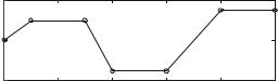
Fig. 4.14 Can you describe the motion?
4.15Motion diagram for a car. Figure 4.13 shows the motion diagram for a car driving along a straight road.
(a) Describe the motion of the car.
(b) Sketch the position as a function of time.
(c) Estimate the velocity of the car throughout the motion.
(d) Estimate the acceleration of the car throughout the motion.
4.16Discover the motion. Figure 4.14 shows the motion diagram for a motion.
(a) Describe the motion qualitatively.
(b) Suggest a process that leads to this motion diagram.
4.17The fastest indian. In the film “The World’s Fastest Indian” Anthony Hopkins plays Burt Munro who reaches a velocity of 201 mph in his 1920 Indian motorcycle. (a) At this velocity, how far does the Indian travel in 10 s?
(b) How long time does the Indian need to travel 1 km?
4.18Meeting trains. A freight train travels from Oslo to Drammen at a velocity of 50 km/h. An express train travels from Drammen to Oslo at 200 km/h. Assume that the trains leave at the same time. The distance from Oslo to Drammen along the railway track is 50 km. You can assume the motion to a long a line.
(a) When do the trains meet?
(b) How far from Oslo do the trains meet?
4.19Catching up. Your roommate sets off early to school, walking leisurely at 0.5 m/s. Thirty minutes after she left, you realize that she forgot her lecture notes. You decide to run after her to give her the notes. You run at a healthy 3 m/s.
(a) What is her position when you start running? (b) What is your position when t < t1?
(c) Sketch the position of you and your roommate as functions of time and indicate in the figure where you catch up with her.
(d) How long time does it take until you catch up with her? (e) How far has she come when you catch up with her?
Now you have developed a strategy to solve such a problem, let us make the problem more complicated and see if you still can use your strategy. First, let us
76 |
4 Motion in One Dimension |
assume that you start off at v0 = 5 m/s, but then you tire gradually, so that your speed drops off with distance, x , reducing your speed by 1 m/s for every hundred meters you run, until you reach a speed of v1 = 2 m/s, which you can keep for a long time.
(f ) Show that your velocity as a function of position can be written as:
|
= |
v1 |
− |
otherwise |
|
v(x ) |
|
v0 |
|
b x when v < v1 = 2 m/s |
(4.80) |
where b = 1 m/s/100 m. (g) Plot or sketch v(x ).
(h) If you know your position and velocity at a time t , how can you find the position and velocity at t + t , a small time-step later?
(i) Write a program to find your position as a function of time. (Remember that you first start running at the time t = t1 = 1800, t ex t s. Before this you are standing still.)
(j) Validate your program by setting b = 0 and comparing the calculated x (t ) with the exact result, xe (t ) = v0(t − t1) when t > t1.
(k) How can you use this result to find where you catch up with your roommate? (l) Where do you catch up with your roommate?
(m) What parts of your solution strategy are general, that is, what parts of your strategy do not change if we change how either person moves?
4.20Electron in electric field. An electron is shot through a box containing a
constant electric field, getting accelerated in the process. The acceleration inside the box is a = 2000 m/s2. The width of the box is 1 m and the electron enters the box with a velocity of 100 m/s.
(a) What is the velocity of the electron when it exits the box?
4.21Archery. As an expert archer you are able to fire off an arrow with a maximum velocity of 50 m/s when you pull the string a length of 70 cm.
(a) If you assume that the acceleration of the arrow is constant from you release the arrow until it leaves the bow, what is the acceleration of the arrow?
4.22Collision. A car travelling at 36 km/h crashes into a mountainside. The crunchzone of the car deforms in the collision, so that the car effectively stops over a distance of 1 m.
(a) Let us assume that the acceleration is constant during the collision, what is the
acceleration of the car during the collision?
(b) Compare with the acceleration of gravity, which is g = 9.8 m/s2.
4.23Braking distance. When you brake your car with your brand new tyres, your acceleration is 5 m/s2.
(a) Find an expression for the distance you need to stop the car as a function of the starting velocity.

4.2 Calculation of Motion |
77 |
With your old tires, the acceleration is only two thirds of the acceleration with the new tyres.
(b) How does this affect the braking distance?
(c) Your reaction time is 0.5 s. If a child jumps into the street 30 m ahead of you when you are driving 50 km/h, are you able to stop with your new tires? What would happen if you did not change tyres?
4.24Motion with constant acceleration. An object starts at x = x0 with a velocity
v = v0 at the time t = t0 and moves with a constant acceleration a0. Show that the velocity v when the object has moved to a position x is v2 − v02 = 2a0(x − x0).
4.25Position plots. The position x (t ) of a particle moving along the x -axis is given in Fig. 4.15.
(a) Indicate in the figure where the velocity of the particle is positive, negative, and zero?
(b) Indicate in the figure where the velocity is maximal and minimal.
(c) Indicate in the figure where the acceleration is positive, negative, and zero?
4.26Velocity plots. The velocity v(t ) of a particle moving along the x -axis is given in Fig. 4.16.
(a) Indicate in the figure where the velocity of the particle is positive, negative, and zero?
(b) Indicate in the figure where the velocity is maximal and minimal.
(c) Indicate in the figure where the acceleration is positive, negative, and zero? (d) Indicate in the figure where the acceleration is maximal and minimal.
4.27Velocity plots. The velocity v(t ) of a particle moving along the x -axis is given in Fig. 4.17.
Fig. 4.15 The position of a particle moving along the
x -axis.
Fig. 4.16 The velocity of a particle moving along the
x -axis.
x [M]
v [M/S]
5
0
-5
0 |
2 |
4 |
6 |
8 |
10 |
t [S]
5
0
-5
0 |
2 |
4 |
6 |
8 |
10 |
t [S]
78 |
4 Motion in One Dimension |
Fig. 4.17 The velocity of a particle moving along the
x -axis
|
20 |
|
|
|
|
|
M/S] |
0 |
|
|
|
|
|
[ |
|
|
|
|
|
|
v |
|
|
|
|
|
|
|
-20 |
|
|
|
|
|
|
0 |
10 |
20 |
30 |
40 |
50 |
|
|
|
|
t [S] |
|
|
(a) Indicate in the figure where the velocity of the particle is positive, negative, and zero?
(b) Indicate in the figure where the particle speeds up and slows down.
(c) Indicate in the figure where the particle is stationary—that is, where it does not move.
(d) Indicate in the figure where acceleration is the largest and the smallest. (e) Sketch the position as a function of time, x (t ).
4.28 A swimming bacterium. When the heliobacter bacteria swims, it is driven by the rotational motion of its tiny tail. It swims almost at a constant velocity, with small fluctuations due to variations in the rotational motion. As a simple model for the motion, we assume that the bacteria starts with the velocity v = 10 µ m/s at the
time t = 0 s, and is then subject to the acceleration, a(t ) = a0 sin(2π t / T ), where a0 = 1 µ m/s2, and T = 1 ms.
(a) Find the velocity of the bacterium as a function of time. (b) Find the position of the bacterium as a function of time.
(c) Find the average velocity of the bacterium after a time t = 10T .
4.29 Resistance. (This problem requires some knowledge of statistics). An electron is moving with a constant acceleration, a0, through a conductor. However, there are many small irregularities in the conductor—called scattering centers. If the electron hits a scattering center it stops, that is, its velocity immediately becomes zero. The scatting centers have a constant density. The probability for the electron to hit a scattering center when it moves a distance x is P = x /b, where b is a length describing the typical length between two scattering centers. Assume that the electron starts from rest. (For simplicity, we measure lengths in nm and time in ns, and you can assume that b = 1 nm and that a0 = 1 nm/ns2). First, we address the case without scattering.
(a) Write a program to find the motion of the electron using Euler-Cromer’s method to find the velocity and position from the acceleration. Plot the position, x (t ), and velocity, v(t ), of the electron as functions of time and compare with the exact result. (b) During the time interval t , the electron moves from x (t ) to x (t + t ). The probability for the electron to stop during this interval is P = (x (t + t ) − x (t ))/b. Explain why the following method models a collision:
4.2 Calculation of Motion |
79 |
dx = x[i+1]-x[i] p = dx/b
if (random.uniform(0,1)<p): v[i+1] = 0
where random.uniform(0,1) produces a random number uniformly distributed between 0 and 1.
(c) Rewrite your program to include the effect of collisions using the algorithm described above. Plot the position, x (t ), and the velocity, v(t ), as functions of time. What do you see? Comment
(d) Find the average velocity vavg for the electron.
(e) How does vavg depend on a0 and b? Can you make a theory that gives the value of vavg ?
(f ) (Requires knowledge of statistics). What is the probability density for the distance, X , between two collisions?
4.30 Ball on vibrating surface. A ball is falling vertically through air over a vibrating surface. The position of the surface is xw (t ) = A cos ωt , where A = 1 cm and ω is called the angular frequency of the vibrations. The ball starts from a position x = 10 cm at t = 0 s. The acceleration of the ball is given as:
|
= |
−g − C (x − xw ) x ≤ xw |
|
|
a(x , v, t ) |
|
−g |
x > xw . |
(4.81) |
where g = 9.81 m/s2 and C = 10000.0 s−2.
(a) Write down the equation you need to solve to find the motion of the ball. Include initial conditions for the ball.
(b) Write down the algorithm to find the position and velocity at ti +1 = ti + t given the position and velocity at ti . Use Euler-Cromer’s scheme.
(c) Write a program to find the position and velocity of the ball as a function of time. (d) Check your program by comparing the initial motion of the ball with the exact solution when the acceleration is constant. Plot the results.
(e) Check your program by first studing the behavior when the vibrating surface is stationary, that is, when A = 0 m and xw = 0 m. Plot the resulting behavior. Ensure that your timestep is small enough, t = 10−5 s. What happens if you increase the timestep to t = 0.02 s?
(f ) Finally, use your program to model the motion of the ball when the surface is vibrating. Use A = 0.01 m, ω = 10 s−1, and simulate 5 s of motion. Plot the results. What is happening?
(g) What happens if you increase the vibrational frequency to ω = 30 s−1?. Plot the results. Can you explain the difference from ω = 10 s−1?

80 |
4 Motion in One Dimension |
Projects
4.31 Sliding on snow. In this project we address the motion of an object sliding on a slippery surface—such as a ski sliding in a snowy track. You will learn how to find the equation of motion for sliding systems both analytically and numerically, and to interpret the results.
We start by studying a simplified situation called frictional motion: A block is sliding on a surface. moving with a velocity v in the positive x -direction. The forces from the interactions with the surface results in an acceleration:
|
|
a |
− |
0 |
|
v = 0 |
, |
(4.82) |
||
|
|
|
= |
|
µ(|v|)g v > 0 |
|
|
|||
|
|
|
µ( |
v |
)g |
v < 0 |
|
|
||
where g = 9.8 m/s |
2 |
|
|
|
| |
| |
|
|
|
|
|
is the acceleration of gravity. Let us first assume that µ(v) = |
|||||||||
µ = 0.1 for the surface. That is, we assume that the coefficient of friction does not depend on the velocity of the block. We give the block a push and release it with a velocity of 5 m/s. (a) Find the velocity, v(t ), of the block.
(b) How long time does it take until the block stops?
(c) Write a program where you find v(t ) numerically using Euler’s or Euler-Cromer’s method. (Hint: You can find a program example in the textbook.) Use the program to plot v(t ) and compare with your analytical solution. Use a timestep of t = 0.01.
The description of friction provided above is too simplified. The coefficient of friction is generally not independent of velocity. For dry friction, the coefficient of
friction can in some cases be approximated by the following formula: |
|
||||||||
µ(v) |
= |
µ |
d + |
µs − µd |
, |
(4.83) |
|||
|
|
1 |
+ |
v/v |
|
|
|||
|
|
|
|
|
|
|
|||
where µd = 0.1 often is called the dynamic coefficient of friction, µs = 0.2 is called the static coefficient of friction, and v = 0.5 m/s is a characteristic velocity for the contact between the block and the surface.
(d) Show that the acceleration of the block is:
a(v) |
= − |
µ |
g |
− |
g |
µs − µd |
, |
(4.84) |
|||
|
d |
|
|
1 |
+ |
v/v |
|
|
|||
|
|
|
|
|
|
|
|
|
|||
for v > 0.
(e) Use your program to find v(t ) for the more realistic model, with the same starting velocity, and compare with your previous results. Are your results reasonable? Explain.
The model we have presented so far is only relevant at small velocities. At higher velocities the snow or ice melts, and the coefficient of friction displays a different dependency on velocity:
4.2 Calculation of Motion |
81 |
− 1 v 2
µ(v) = µm when v > vm , (4.85) vm
where vm is the velocity where melting becomes important. For lower velocities the model presented above with static and dynamic friction is still valid.
(f ) Show that
µ |
µ |
µs − µd |
, |
(4.86) |
|
d + 1 + vm /v |
|||||
m = |
|
|
|
in order for the coefficient of friction to be continuous at v = vm .
(g) Modify your program to find the time development of v for the block when vm = 1.5 m/s. Compare with the two other models above: The model without velocity dependence and the model for dry friction. Comment on the results.
(h) The process may be clearer if you plot the acceleration for all the three models in the same plot. Modify your program to plot a(t ), plot the results, and comment on the results. What would happen if the initial velocity was much higher or much lower than 5 m/s?