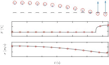
Fig. 10.7 The measured force F (y) as a function of the position y of the top of the cushion. Notice that y is negative when the cushion is compressed

10.3.2 Example: Stopping in a Cushion

You have installed a new soft cushion from SoftCush technology to prevent falling damage. According to the producers, the cushion has been developed to produce a normal force that depends on the compression of the cushion only (and not on the speed of deformation). You do not know the functional form of the force response, F (y), of the cushion, but you have measured the response in a controlled experiment where you pushed the cushion down to a position y and measured the corresponding force F (y). The results are provided in the file cushionforce.d,3 and shown in Fig. 10.7.

Problem: If you jump from a height h and onto the cushion, how far will it compress before you stop? What is the maximum of the force from the cushion on you?

Approach: The cushion reaches its maximum compression when you stop, that is, when your kinetic energy is zero. We will first use the work-energy theorem to find the kinetic energy you have after falling a distance h, and then we will use the workenergy theorem during the contact with the cushion, from you touch the cushion and until you stop.

Sketch and Identify: Figure 10.8 shows an illustration of the forces acting on the person during the jump and a free-body diagram of the person.

Model: We divide the motion into two phases, phase 1 from x0 = h to x1 = 0, where the person is only affected by gravity, G = mg, and phase 2 from x1 = 0 to x2 = −d, where the person is affected by gravity, G, and the force from the cushion, F .

Phase 1: Free fall: In phase 1 the person starts from rest, v0 = 0 and K0 = 0, at a height x0 = h, and reaches the height, x1 = 0 with a velocity, v1, and a kinetic energy, K1.

3http://folk.uio.no/malthe/mechbook/cushionforce.d.

we can solve since the unknown d is the upper limit in the integral. If we knew how to solve the integral analytically, we might have been able to solve the equation, but in this case we only know how to solve the integral numerically. How can we solve such an equation and find the d that satisfies (10.48)?

What we need to do, is to calculate the work:

x

W1,2 = F (x )d x − mgx , (10.49)

0

as a function of the position x of the jumper. Our plan is to vary x until we find a value for x that satisfies the equation, which corresponds to −d. We need to vary x systematically. We start from x = 0, where the jumper comes in contact with the cushion, and then gradually decrease x (remember that the jumper is moving down during the contact with the cushion) until the equation is satisfied, that is, until we find the value for x for which W1,2 is closest to −mgh. More precisely, we make

case we only know the forces F (xi ) for the values xi where it has been measured. Therefore, the best possible resolution we can get is to use the measured xi values as our sequence of xi -values. This means that we start by calculating the work for x1 = x1. Then we calculate the work for x2 = x2, then for x3 = y3 and so on, until, for some value i , the work is approximately equal to −mgh.

How do we calculate the work for x = xk , where k is a number in the sequence of xi values in the datafile? The integral in (10.49) can be calculated using the trapezoidal rule even if we do not know the underlying function—it works well also for a measured dataset:

Numerically, this is done using the function trapz. Here, we only want to do the sum over the first k values of xi , that is, we only want to do the sum from x1 to xk in the list of n such x -values. This corresponds to doing the sum over the first [0:k-1] elements in the position array x:

xval, F = loadtxt(’cushionforce.d’,usecols=[0,1],unpack=True) k = 10

I = trapz(F[0:k-1],x=xval[0:k-1])

We calculate the work for all possible values of k, and store the results in an array work, which gives us the work as a function of k:

from pylab import * m = 80.0 # kg

g = 9.8 # m/sˆ2

x, F = loadtxt(’cushionforce.d’,usecols=[0,1],unpack=True) n = length(x)

work = zeros(n,float) for k in range(1,n-1):

I = trapz(F[0:k],x=-x[0:k]) work[k] = I - m*g*x[k]

plot(y,work,’-b’) xlabel(’x (m)’) ylabel(’W(x) (J)’)

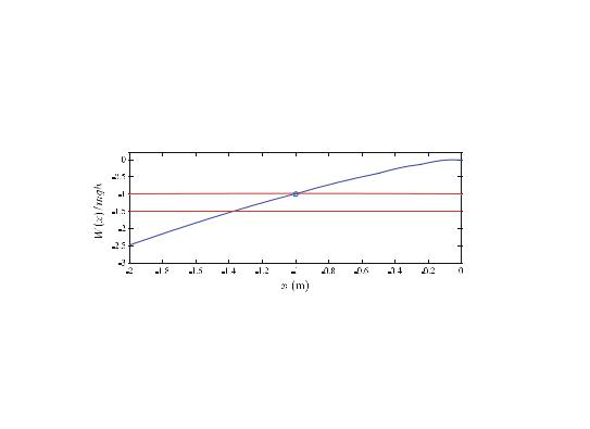
Figure 10.9 shows the work W1,2 as a function of the position x calculated using this program. In the same plot we have also shown the value for −mgh. We see that the work starts at zero and decreases gradually as the deformation increasesa and x becomes a large negative number because the work done is negative: The net work acts to reduce the kinetic energy. When the work reaches the value −mgh the jumper stops: the kinetic energy is now zero. How can we find the x -value this occurs at from our numerical data? Based on the plot, we realize that the x value

smaller than −mgh, but this is a good first approximation. How can we find this value numerically? We use the function find:

i2 = min(find(work<mgh))

x2 = x(i2)

The function find(work<-mgh) returns a list of all the indexes of work that satisfies the condition work<-mgh. We need to find the first of the indexes in this sequence, therefore we take the minimum index in this list, and find the corresponding y-value. We have found the maximum compression of the cushion!

What is the cushion force at this value? This is the corresponding cushion force: F (y2) = 7050 N found by:

>>F2 = F[i2] >>print F2

What would happen if the jumper started from h = 9 m instead? We plot the corresponding value for −mgh in Fig. 10.9. You can read the maximum compression directly from this graph, or determine it numerically as we did above.

Fig. 10.9 Plot of the work W1,2 as a function of the position x of the jumper

10.4 Work Done in Twoand Three-Dimensional Motions

The work-energy theorem was demonstrated for a three-dimensional motion. We have so far studied one-dimensional motions only. How does the application of the theorem change for three-dimensional motion?

Work of Tangential and Normal Forces

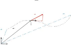
Figure 10.10 illustrates a general three-dimensional motion from 0 to 1. For this motion, the net work is

t1

W = Fnet · v dt = K1 − K0 . (10.51)

t0

Because v points in the tangential direction, we notice that it is only the tangential component of the force that does any work! We can demonstrate this by introducing a local coordinate system along the path of motion, with unit vectors uˆ T in the tangential direction and uˆ N in the normal direction. The velocity vector points along the tangential unit vector:

If we decompose a force, F j , in the tangential and normal directions along the path of motion:

r(t0) r(t)

y

x

290 10 Work

where we have used that the normal unit vector, uˆ N , is normal to the velocity vector, v. Consequently, it is only the tangential component of the force that contributes to the work.

This is also intuitive, since we know that normal forces only contribute to a change in the direction of the velocity vector and not to a change in the speed—it is only the tangential force that can cause a tangential acceleration which causes a change in speed.

Work of a Constant Force in Two and Three Dimensions

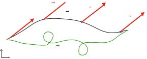
The work done by a constant force has a particularly simple solution. Let us address the work done on an object by a constant force F as the object is moved from r(t0) to r(t1) as illustrated in Fig. 10.11. The work done on the object is

Since the force is constant, we move it outside the integration:

We call s = r = r(t1) − r(t0) the displacement. The work of a constant force is therefore:

x