- •Preface
- •Contents
- •1 Introduction
- •1.1 Physics
- •1.2 Mechanics
- •1.3 Integrating Numerical Methods
- •1.4 Problems and Exercises
- •1.5 How to Learn Physics
- •1.5.1 Advice for How to Succeed
- •1.6 How to Use This Book
- •2 Getting Started with Programming
- •2.1 A Python Calculator
- •2.2 Scripts and Functions
- •2.3 Plotting Data-Sets
- •2.4 Plotting a Function
- •2.5 Random Numbers
- •2.6 Conditions
- •2.7 Reading Real Data
- •2.7.1 Example: Plot of Function and Derivative
- •3 Units and Measurement
- •3.1 Standardized Units
- •3.2 Changing Units
- •3.4 Numerical Representation
- •4 Motion in One Dimension
- •4.1 Description of Motion
- •4.1.1 Example: Motion of a Falling Tennis Ball
- •4.2 Calculation of Motion
- •4.2.1 Example: Modeling the Motion of a Falling Tennis Ball
- •5 Forces in One Dimension
- •5.1 What Is a Force?
- •5.2 Identifying Forces
- •5.3.1 Example: Acceleration and Forces on a Lunar Lander
- •5.4 Force Models
- •5.5 Force Model: Gravitational Force
- •5.6 Force Model: Viscous Force
- •5.6.1 Example: Falling Raindrops
- •5.7 Force Model: Spring Force
- •5.7.1 Example: Motion of a Hanging Block
- •5.9.1 Example: Weight in an Elevator
- •6 Motion in Two and Three Dimensions
- •6.1 Vectors
- •6.2 Description of Motion
- •6.2.1 Example: Mars Express
- •6.3 Calculation of Motion
- •6.3.1 Example: Feather in the Wind
- •6.4 Frames of Reference
- •6.4.1 Example: Motion of a Boat on a Flowing River
- •7 Forces in Two and Three Dimensions
- •7.1 Identifying Forces
- •7.3.1 Example: Motion of a Ball with Gravity
- •7.4.1 Example: Path Through a Tornado
- •7.5.1 Example: Motion of a Bouncing Ball with Air Resistance
- •7.6.1 Example: Comet Trajectory
- •8 Constrained Motion
- •8.1 Linear Motion
- •8.2 Curved Motion
- •8.2.1 Example: Acceleration of a Matchbox Car
- •8.2.2 Example: Acceleration of a Rotating Rod
- •8.2.3 Example: Normal Acceleration in Circular Motion
- •9 Forces and Constrained Motion
- •9.1 Linear Constraints
- •9.1.1 Example: A Bead in the Wind
- •9.2.1 Example: Static Friction Forces
- •9.2.2 Example: Dynamic Friction of a Block Sliding up a Hill
- •9.2.3 Example: Oscillations During an Earthquake
- •9.3 Circular Motion
- •9.3.1 Example: A Car Driving Through a Curve
- •9.3.2 Example: Pendulum with Air Resistance
- •10 Work
- •10.1 Integration Methods
- •10.2 Work-Energy Theorem
- •10.3 Work Done by One-Dimensional Force Models
- •10.3.1 Example: Jumping from the Roof
- •10.3.2 Example: Stopping in a Cushion
- •10.4.1 Example: Work of Gravity
- •10.4.2 Example: Roller-Coaster Motion
- •10.4.3 Example: Work on a Block Sliding Down a Plane
- •10.5 Power
- •10.5.1 Example: Power Exerted When Climbing the Stairs
- •10.5.2 Example: Power of Small Bacterium
- •11 Energy
- •11.1 Motivating Examples
- •11.2 Potential Energy in One Dimension
- •11.2.1 Example: Falling Faster
- •11.2.2 Example: Roller-Coaster Motion
- •11.2.3 Example: Pendulum
- •11.2.4 Example: Spring Cannon
- •11.3 Energy Diagrams
- •11.3.1 Example: Energy Diagram for the Vertical Bow-Shot
- •11.3.2 Example: Atomic Motion Along a Surface
- •11.4 The Energy Principle
- •11.4.1 Example: Lift and Release
- •11.4.2 Example: Sliding Block
- •11.5 Potential Energy in Three Dimensions
- •11.5.1 Example: Constant Gravity in Three Dimensions
- •11.5.2 Example: Gravity in Three Dimensions
- •11.5.3 Example: Non-conservative Force Field
- •11.6 Energy Conservation as a Test of Numerical Solutions
- •12 Momentum, Impulse, and Collisions
- •12.2 Translational Momentum
- •12.3 Impulse and Change in Momentum
- •12.3.1 Example: Ball Colliding with Wall
- •12.3.2 Example: Hitting a Tennis Ball
- •12.4 Isolated Systems and Conservation of Momentum
- •12.5 Collisions
- •12.5.1 Example: Ballistic Pendulum
- •12.5.2 Example: Super-Ball
- •12.6 Modeling and Visualization of Collisions
- •12.7 Rocket Equation
- •12.7.1 Example: Adding Mass to a Railway Car
- •12.7.2 Example: Rocket with Diminishing Mass
- •13 Multiparticle Systems
- •13.1 Motion of a Multiparticle System
- •13.2 The Center of Mass
- •13.2.1 Example: Points on a Line
- •13.2.2 Example: Center of Mass of Object with Hole
- •13.2.3 Example: Center of Mass by Integration
- •13.2.4 Example: Center of Mass from Image Analysis
- •13.3.1 Example: Ballistic Motion with an Explosion
- •13.4 Motion in the Center of Mass System
- •13.5 Energy Partitioning
- •13.5.1 Example: Bouncing Dumbbell
- •13.6 Energy Principle for Multi-particle Systems
- •14 Rotational Motion
- •14.2 Angular Velocity
- •14.3 Angular Acceleration
- •14.3.1 Example: Oscillating Antenna
- •14.4 Comparing Linear and Rotational Motion
- •14.5 Solving for the Rotational Motion
- •14.5.1 Example: Revolutions of an Accelerating Disc
- •14.5.2 Example: Angular Velocities of Two Objects in Contact
- •14.6 Rotational Motion in Three Dimensions
- •14.6.1 Example: Velocity and Acceleration of a Conical Pendulum
- •15 Rotation of Rigid Bodies
- •15.1 Rigid Bodies
- •15.2 Kinetic Energy of a Rotating Rigid Body
- •15.3 Calculating the Moment of Inertia
- •15.3.1 Example: Moment of Inertia of Two-Particle System
- •15.3.2 Example: Moment of Inertia of a Plate
- •15.4 Conservation of Energy for Rigid Bodies
- •15.4.1 Example: Rotating Rod
- •15.5 Relating Rotational and Translational Motion
- •15.5.1 Example: Weight and Spinning Wheel
- •15.5.2 Example: Rolling Down a Hill
- •16 Dynamics of Rigid Bodies
- •16.2.1 Example: Torque and Vector Decomposition
- •16.2.2 Example: Pulling at a Wheel
- •16.2.3 Example: Blowing at a Pendulum
- •16.3 Rotational Motion Around a Moving Center of Mass
- •16.3.1 Example: Kicking a Ball
- •16.3.2 Example: Rolling down an Inclined Plane
- •16.3.3 Example: Bouncing Rod
- •16.4 Collisions and Conservation Laws
- •16.4.1 Example: Block on a Frictionless Table
- •16.4.2 Example: Changing Your Angular Velocity
- •16.4.3 Example: Conservation of Rotational Momentum
- •16.4.4 Example: Ballistic Pendulum
- •16.4.5 Example: Rotating Rod
- •16.5 General Rotational Motion
- •Index
356 |
12 Momentum, Impulse, and Collisions |
Newton’s Second Law
We have previously introduced Newton’s second law of motion as: |
|
|
|
Fextj = ma . |
(12.16) |
j
However, the most fundamental, and the original, form of Newton’s second law is:
|
|
d |
|
|
Fextj |
= |
|
p , |
(12.17) |
|
||||
|
|
dt |
|
j
The net force acting on an object causes a change in the momentum of the object.2 For an object with constant mass, this formulation reduces to the original formu-
lation:
|
|
d |
d |
dm |
dv |
|
||||
Fextj |
= |
|
p = |
|
(mv) = |
|
v + m |
|
= ma . |
(12.18) |
|
|
|
|
|||||||
|
|
dt |
dt |
dt |
dt |
|
j |
|
|
|
|
=0 |
This law is a fundamental principle in physics, on the same level as the energyprinciple. It is the general formulation of Newton’s second law, and we use the term Newton’s second law for this law as well as the special case when the mass is constant.
12.3 Impulse and Change in Momentum
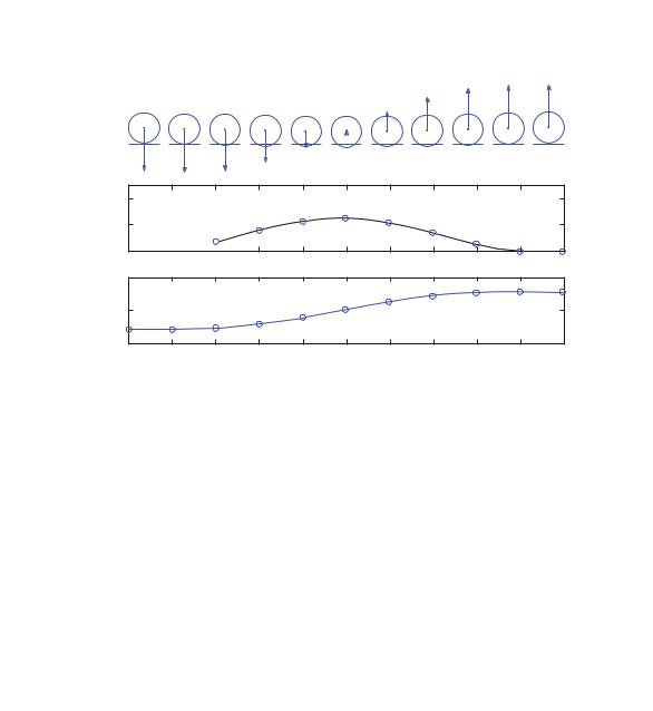
What is causing a change in the momentum of an object? Let us study an object that is affected by a force during a short time interval, such as a tennis ball during a serve. While the ball is in contact with the racket, the contact force F(t ) on the ball varies as illustrated in Fig. 12.2. When the racket makes contact with the ball, the contact force is small, but it grows rapidly as the racket deforms against the ball. As the ball speeds up, the force decreases while the racket returns to its original shape, until the force reaches zero as the ball leaves the racket.
During the collision, other forces such as gravitational forces are negligible compared with the contact force from the racket. We can therefore assume that the contact force F(t ) is approximately equal to the net force on the ball.
The change of momentum of the ball from the time t0 before contact with the racket to the time t1 after the ball has left the racket is
p = p2 − p1 |
= |
|
t1 |
dt |
dt = |
F(t ) dt . |
(12.19) |
|
|
|
dp |
|
t1 |
|
|
|
|
|
t0 |
|
|
t0 |
|
2This formulation of Newton’s second law can also be exteded to relativistic mechanics.
12.3 Impulse and Change in Momentum |
357 |
|
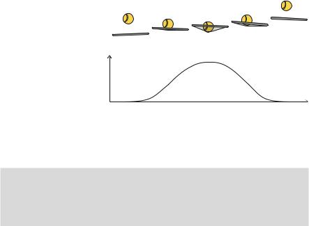
Fig. 12.2 Illustration a ball |
|
|
being hit by a tennis racket, |
|
|
showing an illustration of the |
|
|
collision as a function of |
|
|
time, and a plot of the force |
|
|
F (t ) from the racket on the |
|
|
ball as a function of time |
F(t) |
|
|
|
|
|
|
t |
The left side is the change in momentum of the ball. The right side includes both the strength of the interaction—the force F—and the duration of the interaction. We call this quantity the impulse, J, experienced by the object during the collision:
Impulse:
t1
J = |
Fnet(t ) dt . |
(12.20) |
t0
If the direction of the net force F(t ) does not change during the collision, the impulse is directed in the same direction as F(t ). In this case, the impulse, J , is the area under the curve, F (t ), in Fig. 12.2.
Time-Averaged Force
Unfortunately, we generally do not know the time dependency of the net force, since this requires a detailed force model for the collision, or a detailed measurement of the forces acting. Instead, we can use our knowledge of the change in momentum to determine the average force acting on the ball during the collision. The time-average force is defined as:
Favgnet = Fext(t ) = t1 − t0 |
t0 |
F(t ) dt . |
(12.21) |
1 |
t1 |
|
|
where t = t1 − t0 is the duration of the collision. We define the start of the collision as the time t0 when the ball comes in contact with the racket (when the contact force becomes non-zero), and the end of the collision as the time t1 when the ball loses contact with the racket (when the contact force becomes zero). We recognize the
358 |
12 Momentum, Impulse, and Collisions |
F [ N ]
30
25
20
15
10
5
0
0 |
0.01 |
0.02 |
0.03 |
0.04 |
0.05 |
0.06 |
0.07 |
0.08 |
0.09 |
0.1 |
t [ s]
Fig. 12.3 A plot of the force, F (t ), as a function of time during a collision, and the average force Favg. In most cases, the average force is a good estimate for the typical force and the maximum force during the collisions
integral on the right-hand side as the impulse of the net force, which is equal to the change in momentum:
Favgnet = |
t |
|
F(t ) dt = |
t J = |
t |
p . |
(12.22) |
|
|
1 |
|
t1 |
1 |
|
1 |
|
|
|
|
|
t0 |
|
|
|
|
|
Momentum Change During a Collision
The momentum change during a collision gives useful insight into the collision: While the net force may vary throughout the collision, and the maximum force may be much larger than the average force, the average force is still a reasonable estimate for the force acting on the object. For example, if we want to estimate the damage done to an object during a collision, the average force is a good estimate also of the maximum force, because for most physical interactions (for most force models), the force does not display a very narrow peak, but instead varies gradually over a wider time interval, and hence the maximum force is often just a few times the maximum force. (See Fig. 12.3 for an illustration).
Test your understanding: You jump down from a window 5 meters above the ground. How should you land in order to minimize the force on you from the ground? What determines the change in momentum during the impact? Demonstrate that you can answer this question using both energy and momentum considerations.
12.3.1 Example: Ball Colliding with Wall
Problem: A ball falls vertically and collides with a horizontal floor. The force from the floor on the ball during the contact is:
12.3 Impulse and Change in Momentum |
359 |
y
F
G
t
t0 |
t1 |
t2 |
Fig. 12.4 Free-body diagram for a ball colliding with a floor
N = k (R |
0 y) |
3/2 |
y ≥ R |
(12.23) |
|
− |
y < R |
|
You can neglect air drag. Find the motion of the ball and visualize the change in momentum during the collision.
Model: We describe the motion of the ball by its vertical position, y(t ). The ball is affected by two forces, the contact force N and gravity, G, as illustrated in Fig. 12.4, where we have neglected air drag.
We find the acceleration of the ball from Newton’s second law. The forces acting on the ball are the contact force from the surface and gravity:
ma = F net |
1 |
N − g . |
(12.24) |
|
= N − mg a = |
|
|||
|
m
Solve: The ball starts at y(t0)y0 with the velocity v(t0) = v0. While we may be able to find the motion y(t ) analytically, a numerical approach based on Euler-Cromer’s method is sufficient. This is implemented in the following program:
from pylab import * g = 9.8 # m/sˆ2
R= 0.02 # m m = 0.1 # kg
y0 = 0.021 # m
v0 = -2.8 # m/s k = 1000000.0 # time = 0.005 dt = 0.00001
n = int(round(time/dt)); t = zeros(,n,1);
y = zeros(n,1); v = zeros(n,1);
Fnet = zeros(n,1); y[0] = y0
v[0] = v0
for i in range(n): dy = R-y[i]
if (dy<=0.0): N = 0.0
else:
N = k*dy**1.5
360 |
12 Momentum, Impulse, and Collisions |
pY [kgm/s] F [N]
400
200
0
0.5
0
−0.5
0 |
0.5 |
1 |
1.5 |
2 |
2.5 |
3 |
3.5 |
4 |
4.5 |
5 |
|
|
|
|
|
t [s] |
|
|
|
|
x 10−3 |
Fig. 12.5 Illustration of a simulation of a ball bouncing on the floor
Fnet[i] = N - m*g a = Fnet[i]/m
v[i+1] = v[i] + a*dt y[i+1] = y[i] + v[i+1]*dt t[i+1] = t[i] + dt
subplot(2,1,1), plot(t,Fnet) xlabel(’t [s]’),ylabel(’F [N]’) p = m*v
subplot(2,1,2), plot(t,p)
xlabel(’t [s]’), ylabel(’P [kgm/s]’)
Figure 12.5 illustrates a simulation with this model. Here, you can see the time development of the net force and the momentum of the ball throughout the collision.
Change in momentum: What is the change in momentum of the ball? Since the force only depends on the position of the ball, the force is conservative and the mechanical energy of the ball is conserved throughout the collision. Hence, the kinetic energy of the ball is the same when the ball comes in contact with the surface and when it loses contact with the surface, since the vertical position is the same:
E0 = U (y0) + |
1 |
mv2 |
= E1 = U (y1) + |
1 |
mv2 |
, |
(12.25) |
||||
|
|
|
|||||||||
|
|
|
|||||||||
|
2 |
0 |
|
|
|
|
2 |
1 |
|
|
|
|
|
|
|
|
|
|
|
|
|||
where y0 = y1 and therefore |
1 |
|
|
1 |
|
|
|
|
|
|
|
|
mv2 |
= |
mv2 |
, |
|
|
|
|
(12.26) |
||
|
|
|
|
|
|
|
|||||
|
|
|
|
|
|
|
|||||
|
2 |
0 |
|
2 |
1 |
|
|
|
|
|
|
|
|
|
|
|
|
|
|
|
|
which gives v1 = −v0, since we know that the velocity after the collision is in the opposite direction of the velocity before the collision.