Добавил:
Опубликованный материал нарушает ваши авторские права? Сообщите нам.
Вуз: Предмет: Файл:
Elementary Mechanics Using Python- 2015.pdf
Скачиваний:
1
Добавлен:
07.04.2024
Размер:
7.83 Mб
Скачать

7.5 Force Model—Spring Force

201

7.5.1 Example: Motion of a Bouncing Ball with Air Resistance

In this example we study the motion of an object subject to a constant force, a velocitydependent force, and a position-dependent force. We solve the problem numerically and discuss the results following a workflow similar to what you will find in many practical problems.

Let us continue to refine the description of a ball thrown in the classroom. So far we have introduced gravity and air resistance. But what happens when the ball hits the floor? We need to also include a force model for the normal force from the floor on the ball. The simplest approach to such a contact force model is a spring model: We model the interaction between the floor and the ball as a single spring. But the normal force is zero when there is no contact. In this problem we demonstrate how to include such effects in our models.

Problem: A ball is thrown from a height h above the ground with an initial velocity v0. Find the velocity and position of the ball as a function of time t . Include the normal force from the floor while the ball is in contact with the floor.

Identify and Sketch: We describe the position of the ball by r(t ), measured in a coordinate system with origin at the floor. The initial position and velocity of the projectile is r(t0) = h j and v(t0) = v0 = vx ,0 i + vy,0 j.

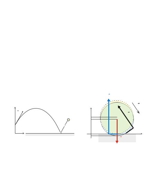
Model: The motion of the ball is determined by the forces acting: air resistance, FD , the normal force N from the floor, and gravity, G = −mg j, as illustrated in the free-body diagram in Fig. 7.10. We use a square law for air resistance:

FD = −Dvv .

(7.47)

The normal force from the floor on the ball is represented by a spring force. This is a strong simplification of the actual deformation process occurring at the contact between the ball and the floor due to the deformation of both the ball and the floor.

(A)

N

(B)

y

v

y

v0

FD


y

h


x

x


G

Fig. 7.10 a Sketch of the path of the ball. b Free-body diagram for the ball when in contact with the floor

202 7 Forces in Two and Three Dimensions

The deformed region corresponds roughly to the region of “overlap” between the ball and the floor in Fig. 7.10. The depth of this region is y = R y(t ), where R

is the radius of the ball, which corresponds to the compression

L of the spring:

N = −k ( R y(t )) j .

(7.48)

We check that the sign is correct: The normal force must act upward when y < R, hence the sign must be negative.

However, we must also ensure that the normal force only acts when the ball is in contact with the floor, otherwise the normal force is zero. The full formation of the

normal force is therefore:


N =


0

when y(t ) ≥ R .

(7.49)


k ( R y(t )) j

when y(t ) <

R


Newton’s second law: Newton’s second law is now


F j = G + FD + N = ma ,


(7.50)


j


which gives


a = − ( D/m) v v g j + N/m ,


(7.51)

with the initial conditions: r(t0) = r(0 s) = r0 and v(t0) = v(0 s) = v0. While it is difficult to determine the motion analytically, we may be able to find analytical solutions for parts of the motion. However, we can determine the motion numerically by integrating (7.51) using Euler-Cromer’s method:


v(ti +

t ) v(ti ) +

t a(ti , r(ti ), v(ti ))

(7.52)


r(ti +

t ) r(ti ) +

t v(ti + t ) .

(7.53)

The implementation is straight-forward:


from pylab import *


m = 0.2

# kg


g = 9.81

# m/sˆ2


vT = 20.0

# m/s


h = 2.0

# m


R = 0.1

# m


k = 1000.0

# N/m


r0 = array([0.0,h])


v0 = array([10.0,10.0])


time = 20.0

# s


dt = 0.001

#


s n = int(round(time/dt)) r = zeros((n,2),float)

v = zeros((n,2),float) t = zeros(n,float) r[0] = r0

v[0] = v0

7.5 Force Model—Spring Force

Fig. 7.11 Plot of the trajectory of the ball calculated using Euler-Cromers method for quadratic air resistance (solid line), compared with the trajectory without air resistance (dashed line)

y [M]

203

6

4

2

0


0

5

10

15

x [M]

t[0] = 0.0

# Simulation loop for i in range(n): if (r[i,1]<R):

N = k*(R-r[i,1])*array([0,1]) else:

N = array([0,0])

FD = - D*norm(v[i])*v[i] G = -m*g*array([0,1]) Fnet = N + FD + G

a = Fnet/m

v[i+1] = v[i] + a*dt r[i+1] = r[i] + v[i+1]*dt t[i+1] = t[i] + dt

plot(r[:,0],r[:,1])

xlabel(’x [m]’), ylabel(’y [m]’)

where we have used the vT = 10.0 m/s to calculate D, and m = 0.2 kg. We have chosen to use the spring constant k = 1000 N/m, a number we have largely guessed for now. (The effective spring constant may be measured by experiment or calculated if we know the material properties of the ball and the floor). The resulting path is illustrated in Fig. 7.11, where it is compared with the path of the ball without air resistance.

Detailed analysis of wall contact: While the behavior in Fig. 7.11 looks reasonable at first, a closer examination shows that something is wrong, at least according to our intuition. When there is no air resistance, the ball bounces back to the same height! We know that a real ball would not behave like this. What is wrong?

Figure 7.12 shows a magnification of the behavior of the ball during a bounce when there is no air resistance. The red lines in the figures mark the positions and the times when the ball comes in contact with the floor. We see that the horizontal velocity, vx , does not change at all during the bounce. This is not surprising, since the normal force only has a vertical component. No horizontal forces means no horizontal acceleration. However, we also see that the vertical velocity component, vy , simply reverses during the bounce. This is the part that strikes us as unrealistic. And indeed it is. How can we modify the force model for the normal force to ensure that the vertical speed is smaller after the collision? This question we will return to later when we discuss energy and collisions. The short answer is that we need to introduce a force that is velocity dependent: Any force model that only depends on

204

0.2


[M ]


0.1


y


0


3.6

[M /S ]

3


2


X


v


1


20


[M /S ]

0


Y


v


−20

7 Forces in Two and Three Dimensions

3.8

4

4.2

4.4

4.6

4.8

5

5.2

x [M ]

2.21

2.22

2.23

2.24

2.25

2.26

t [S ]

2.21

2.22

2.23

2.24

2.25

2.26

t [S ]

Fig. 7.12 Plot of the trajectory of the ball without air resistance during its collision with the floor. The red lines illustrates the points where the ball comes in contact with the floor

the vertical position y(t ) of the ball will always result in a reversal of the velocity! By introducing a viscous force, a linear velocity dependent force model, during the collision with the floor, the outgoing vertical velocity will be reduced. But more on this later! (See Chap. 12.)

Comments: We have now built a model for a bouncing ball, including both air resistance and a normal force from the floor. You should notice the simple structure followed systematically: as long as we can develop force models for the interactions, we can model the motion. This method is robust and no different in one-, two-, or three dimensions. You should also notice that the normal force changes: It does not always just balance the gravitational force—it is indeed larger than the gravitational force in parts of the collision. Otherwise the normal force would not be able to change the direction of the ball. This simple point is a clear result of the force model approach, and also of a careful physical analysis, but represents a classical misunderstanding.