9.1.1 Example: A Bead in the Wind

FD,x = FD · i = −kv (v − w) · i = −kv (v · i − w · i) = −kv (0 − w) = kvw

We also notice that the normal force, N, only has a component along the x -axis. We have now decomposed the forces, and can apply Newton’s second law along the x - and y-directions.

Since the bead is constrained not to move in the x -direction, we know that the acceleration in the x -direction is zero. Newton’s law along the x -axis therefore gives:

The normal force is therefore constant for this particular model of the motion!

We find the acceleration of the bead by applying Newton’s law in the y-direction:

From these equations you know how to find the motion of the bead. For this particular formulation of the problem, it is decoupled—the motion of the bead in the y-direction does not depend on the wind velocity.

Test your understanding: How would this problem change if you used a square-law for the air drag?

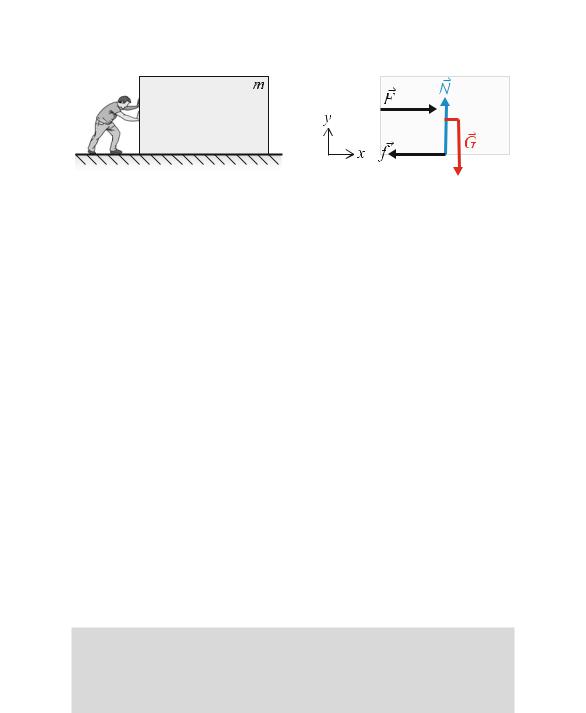
9.2 Force Model—Friction

We have now addressed constrained motion such as the motion of a block sliding along a surface as illustrated in Fig. 9.6. We have shown that we can use Newton’s second law in combination with the constraint to determine the normal force on the block without including a force model for the contact. For the case illustrated in Fig. 9.6, we can apply Newton’s second law in the vertical direction to find:

Fig. 9.6 Left Illustration of a crate on the floor. Right A free-body diagram of a crate on the floor. You are trying to push the crate with the force F directed along the floor

But so far there has been no coupling between the forces normal to the surface and the forces along the surface—the tangential forces. The magnitude of the normal force has no impact on the motion of the block.

In real systems there are several mechanisms that introduce a coupling between the normal and tangential forces. When we discuss macroscopic systems it is common to group these mechanisms into a common term: friction. Friction is a force acting on the contact between two objects, it acts tangential to the contact, and it depends on the magnitude of the normal force at this contact. The introduction of a force model for friction forces is therefore essential in order to get a realistic description of contact forces. Unfortunately, the concept of friction is not that well defined. The mechanisms of friction are currently not well understood, and are subjects of current research. There is also not only one, single mechanism responsible for the tangential forces acting on a contact—there are many different mechanisms acting all at the same time, including effects such as surface geometry and roughness, the effect of thin fluid films, surfactants, and dirt on the surfaces, the effect of adhesion forces and plastic deformation of small asperities on the contact surface, the effect of the external boundaries, and many more. In addition, it is also clear that the scale you are studying is important: For example on very small scales inter-atomic forces and the presence of individual atoms or molecules along the surface can affect the tangential forces acting.

But wait, you interrupt, I already know something about friction, and it is a simple law! Yes. Already in 1699 Amontons reported the experimental observations that we today also call the “laws of friction”:

Amonton’s laws of dynamic friction:

•The friction force is proportional to the normal force: F = µN .

•The friction force does not depend on the apparent contact area.

This is an experimental observation that turns out to be surprisingly robust, in particular considering that it includes so many different effects! In this section we will motivate and discuss the force model for friction as a contact force acting in the tangential direction along any contact between two solids. We will introduce a model for

the static friction force for the case when the two surfaces are not moving relative to each other, and a model for the dynamic friction force when the surfaces are moving relative to each other.

Static Friction

We all have a good intuition for solid friction because it is an important force in our macroscopic world. If you want to push a heavy crate along the floor, you know that you need to apply a certain force to “get it going”. If you do not push hard enough, it will not start moving. You may also know that if you want to keep it moving, you must constantly apply a force to it, otherwise it will stop moving. If you give the crate a hard push, it will start moving, but you know that it will decelerate and stop after some distance. These simple insights provides us with some of the basic properties of a the friction force

Sliding box model system: Let us analyze the motion of a crate on a flat floor in detail (See Fig. 9.6 for an illustration). You push on the crate with a horizontal force, F. The motion of the crate is determined by the forces acting on it: The applied force, F, the normal force N from the floor, and the gravitational force, G. The crate is cannot move down through the floor—it is constrained not to move in the y-direction. We can therefore use Newton’s second law in the y-direction to determine the normal force:

We also know, from our experience or from staging a simple experiment, that when the applied force, F, is small, the crate is not moving in the horizontal direction. However, according to Newton’s second law of motion the horizontal acceleration is given by the net horizontal force:

Because the crate is not moving, the sum of the forces must be zero. Consequently, the crate cannot only be affected by the applied force F in the horizontal direction. There must be an additional force, counteracting the applied force. This force must come from the contact with the floor. And the force has the apparently “magical” property that it is exactly equal to the applied, horizontal force! If you push with a very small force, F0, then the force from the floor will be exactly the same but in the opposite direction. If you push with a slightly larger force, F1, then the force from the floor will again be exactly the same, but in the opposite direction. In this respect the friction force is similar to the normal force from the floor on the crate, which in the static situation matches the force from gravity. We call the force from the floor on the crate the static friction force

Microscopic model for static friction: The word static indicates that it is the friction along a surface when the object does not move relative to the surface. We can develop a simple model for the origin of the static friction force from a microscopic picture of the contact. On the microscopic scale, the contact between the crate and the floor consists of many, small irregularities: small bumps on the surface of the floor and the surface of the crate. When the crate is placed on the surface, these irregularities are pressed together. One possible explanation is that in this process, the irregularities are “glued” together due to adhesive forces between the two materials. This glue acts like small springs, so that when we try to push at the crate, these small springs are extended, exerting forces that counteract the applied force. However, if the applied force on the crate becomes too large, the adhesive forces become so large that the contacts break, and the crate starts to slip.

It is reasonable to assume that the number of irregularities that are in contact, and possibly the contact area of each irregularity, increase with the normal force. This means that we should discern between the apparent area of contact, which is simply the size of the side of crate facing the floor, and the actual area of contact, which is given by the contact areas of all the small irregularities. If the actual contact area is proportional to the normal force, we expect the static friction force also to be proportional to the normal force.

The simple model we have developed now, based only on our intuition, is surprisingly close to the most usual description of static friction. By the word “law” here, we mean a model for the force — it is not a fundamental law of nature, but rather a model that can often, but not always, be applied to contact problems.

Coefficient of static friction: The upper limit of the static friction force is Fm = µs N , where N is the normal force for the contact, and µs is called the coefficient of static friction. If the friction force exceeds this upper limit, the object will start moving relative to the surface, and our model for static friction is no longer valid.

We see that the concept of static friction is closely related to a constraint on the motion of an object:

The static friction force is a tangential force acting on the interface between two solids in contact that are not moving relative to each other. The magnitude and direction of the force is so that the two object do not accelerate relative to each other. However, there is an upper limit on the magnitude of the static friction force

where N is the normal force at the contact.

In order to determine the static friction force we need to assume that the objects are not accelerating, that is, we need to assume a constraint on the motion, and use Newton’s second law of motion to determine the static friction force. Then, we need

Fig. 9.7 Left Illustration of a crate moving along the floor. Right A free-body diagram of a crate on the floor. You are pushing the crate with the force F directed along the floor

to check that the force does not exceed the threshold. If it exceeds the threshold, the objects will start moving relative to each other, and we need another force model—the dynamic friction model.

This law is experimentally justified and it is only an approximation of the real behavior of materials, where many different effects contribute to bring about the effect of a static friction force.

Dynamic Friction

You are gradually increasing how hard you are pushing a crate on the floor. What happens when the crate slips? Our model so far has been for static friction. However, you know from your own experience that if you give the crate an initial velocity and release it along the floor, it slows downs and stops (see Fig. 9.7). That means that the crate decelerates. We can therefore use Newton’s second law and conclude that because the crate decelerates, there must be a force acting along the floor in the direction opposite the movement, which is the cause of the deceleration. We call this force the dynamic friction force.

There is a surprisingly simple law for the dynamic friction force, Fd , acting on an object in contact with another object:

The dynamic friction force, Fd , is tangential to the surface of contact. The magnitude of the force is Fd = µd N where N is the normal force across the

contact. The direction of the force is opposite the relative motion of the two objects.

This law is empirically based. This means that it is the result of measurements. The law states that the dynamic friction force depends only on the normal force and on the coefficient of friction, which is a property of the two materials in contact. The dynamic friction force does not depend on the area of contact. Neither does it depend on the velocity of the object relative to the floor. This is surprising—we