328 Radio Engineering for Wireless Communication and Sensor Applications

Dt . The position of the plane is obtained from the measured azimuth, elevation, and distance.

Traffic-alert and collision-avoidance systems (TCAS) are based on transponders, which warn pilots about potential midair collisions. There are three versions of the system: TCAS I indicates potential threats, TCAS II gives simple advice such as ‘‘climb’’ or ‘‘descend,’’ and TCAS III gives more detailed advice.

12.6 Radar

The technique to detect and locate reflecting objects—targets—by using radio waves was first called radio detection and ranging [8]. Eventually, this expression was reduced to the acronym radar. The serious development of radar began in the mid-1930s and progressed rapidly during World War II.

The applications of radar are numerous: Surveillance radar is used in air-traffic control; tracking radar continuously tracks aircraft or missiles; weather radar reveals rain clouds and their movements; police speedometers are used in traffic control; collision-avoidance radar may be installed on all kinds of vehicles; surface-penetrating radar can locate buried objects or interfaces beneath the Earth’s surface or within visually opaque objects; and so on. Radar is applied in navigation (Section 12.5), in remote sensing of the environment (Section 12.7), in radio astronomy (Section 12.8), and in various sensors (Section 12.9).

Radar is either monostatic or bistatic. In monostatic radar the same antenna transmits and receives; in bistatic radar these are at separate locations. According to the waveforms used, radar can be divided into pulse radar, Doppler radar, and frequency-modulated radar. The basic principles of these different types of radar and the surveillance and tracking radar are treated in this section.

12.6.1 Pulse Radar

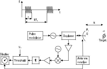
Pulse radar transmits a repetitive train of short-duration pulses, which reflect from the target back to the receiver. The distance to the target can be calculated from the speed of radio waves in the medium, which in most cases is with a good approximation of the speed of light in vacuum and the time Dt it takes for the pulses to propagate back and forth:

330 Radio Engineering for Wireless Communication and Sensor Applications

to an adjustable threshold voltage, VT . An output voltage higher than VT is interpreted as a target. A too-low VT increases the probability that noise is interpreted as a target; a too-high VT reduces the probability of observing a weak target. The display may be a plan position indicator (PPI), in which the echo signal modulates an electron beam rotating synchronously with the antenna. Thus, the display shows the surroundings of the radar in polar form.

The power density produced by the radar at a distance of R is

where Pt is the transmitted power (during a pulse) and G is the gain of the antenna. The radar cross section of a target, s, is the fictional area intercepting that amount of power that, when scattered equally in all directions, produces an echo at the radar equal to that from the target. In other words,

s = power reflected towards radar/unit solid angle incident power density/4p

The radar cross section of a target depends on the frequency and polarization, as well as on the direction of observation. In case of monostatic radar, the power density produced by the target at the radar is (same R in both directions)

and the power received is (same G both in transmitting and receiving mode)

If Pr , min is the minimum received power, which is reliably interpreted as a target, the maximum operating range of the radar is

This equation is called the radar equation. Because of the two-way propagation loss, doubling the transmitted power increases the maximum range only by 19%.

The minimum power Pr , min or the sensitivity of the radar is

where TS is the system noise temperature, Bn is the noise bandwidth of the receiver, and S /N is the signal-to-noise ratio corresponding to the threshold voltage. Usually the IF filter determines the noise bandwidth, which should be about 1/t . If the bandwidth were narrower, the received pulses would distort. If it were broader, the sensitivity would be reduced.

The radar equation (12.6) is based on many idealizations. The atmospheric attenuation reduces the maximum operating range, especially at high microwave and millimeter-wave frequencies. The radar cross section of the target often changes rapidly, fluctuates, and thus has a statistical nature. Also noise and other interfering signals are statistical. Therefore, instead of exact figures, only probabilities can be estimated for a given radar measuring a target of a given type. The maximum operating range for radar may be calculated by assuming a certain probability of detection and a certain probability of false alarms.

The performance of pulse radar may be improved considerably by pulse integration, pulse compression, and moving target indication. Even if the beam of the antenna is scanning rapidly, several pulses are received from a target during each scan. The sensitivity of the radar can be improved by summing these pulses. The summing, or integration, is performed either coherently at IF or noncoherently after detection. An ideal coherent integration of n pulses having equal amplitudes improves the S /N by a factor of n . A noncoherent integration is not as effective as the coherent integration but it is much simpler to realize.

In pulse compression, the transmitted pulse is long and its carrier frequency or phase is modulated. In the receiver, the pulse is then compressed to a short impulse, for example, by using a filter whose delay is frequency dependent. Pulse compression combines the advantages of high-energy pulses and short pulses, that is, a large operating range and a good resolution.

The echoes originating from fixed objects in the radar’s surroundings, clutter, may mask the detection of more interesting weak targets. The effect of clutter may be reduced by the use of a moving target indicator (MTI). Figure 12.16 shows the principle of a simple MTI in which echoes of