

222 Radio Engineering for Wireless Communication and Sensor Applications
produced by the driven and parasitic elements add in phase in the forward direction and cancel in the reverse direction.
The driven element of a Yagi antenna is in a resonance, that is, the input impedance is resistive, when the length of the element is 0.45 to 0.48 wavelength. The driven element is often a folded dipole. The reflector is 0.15 to 0.30 wavelength behind the driven element and it is about 5% longer than the driven element. The directors are about 5% shorter than the driven element and their spacings are 0.15 to 0.30 wavelength. Often the directors have equal lengths and equal spacings, although the optimization of dimensions would give a slightly higher directivity. A larger number of director elements means a higher directivity. Usually there are three to twelve directors. The directivity of a seven-element Yagi is typically 12 dB. The narrow bandwidth is a drawback of the Yagi antenna. In a cold climate snow and ice covering the elements may easily spoil the directional pattern.
A log-periodic antenna is a broadband antenna whose properties repeat at frequencies having a constant ratio of t. The structure is periodic so that if all the dimensions are multiplied or divided by t, the original structure, excluding the outermost elements, is obtained. Figure 9.14 shows a logperiodic dipole antenna. The antenna is fed from the high-frequency end, and the feed line goes through all elements, so that the phase is reversed from an element to the next one. Only the element being in resonance radiates effectively. The element behind it acts as a reflector and the element in front of it acts as a director. Thus, the active part of the antenna depends on the frequency. The directivity is typically 8 dB.
9.5 Other Wire Antennas
A loop antenna is a circular or rectangular wire, which may consist of several turns. If the loop is small compared to a wavelength, the current is nearly
Figure 9.14 Log-periodic dipole antenna.

Antennas |
223 |
constant along the loop. The maximum of the directional pattern is in the plane of the loop and the nulls are perpendicular to that plane as in Figure 9.15(a). The pattern is like the pattern of a small dipole having the electric and magnetic fields interchanged. Therefore, a small loop can be considered to be a magnetic dipole. The radiation resistance is
|
Sl2 |
D |
|
|
|
R r = 320p4 |
|
NA |
2 |
V |
(9.30) |
|
|
|
|||
where A is the area of the loop and N is the number of turns.
The current of a larger loop is not constant. Then the directional pattern differs from that of a small loop. If the length of the circumference is one wavelength, the maximum of the directional pattern is perpendicular to the plane of the loop and the null is in the plane of the loop. Figure 9.15(b) shows a quad antenna, which is made of such loops. Like the Yagi antenna, the quad antenna has a driven element, a reflector, and one or more directors. Quad antennas operating at different frequency ranges can be placed inside each other because the coupling of such loops is small.
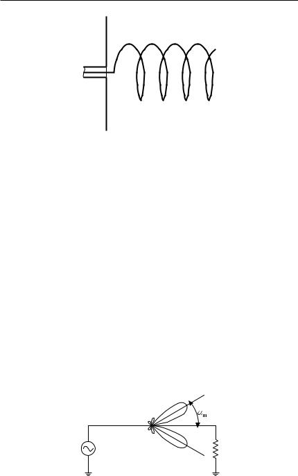
A helix antenna, shown in Figure 9.16, is a helical wire having either the left-handed or right-handed sense. If the length of the circumference L is less than l/2, the helix antenna radiates in the normal mode; that is, the maximum of the directional pattern is perpendicular to the axis of the helix. This kind of a helix antenna operates as a shortened monopole, except the field is elliptically polarized. If L is from 0.75l to 1.25l, the helix antenna operates in the axial mode; that is, the main beam is along the axis of the helix and the field is circularly polarized.
Long-wire and rhombic antennas are traveling-wave antennas, which are used at HF range. The current has constant amplitude but the phase changes linearly along the wire (in a dipole antenna, the amplitude of the current changes but the phase is constant).
Figure 9.15 (a) Small loop antenna and its directional pattern; and (b) quad antenna.
224 Radio Engineering for Wireless Communication and Sensor Applications
Figure 9.16 Helix antenna fed from a coaxial cable through a conducting plane.
The long-wire antenna is usually a horizontal wire, which is terminated with a matched load, as shown in Figure 9.17. The conical directional pattern is
En (a) = |
|
sin a |
sin [pL (1 |
− cos a)/l] |
(9.31) |
|
1 |
− cos a |
|||||
|
|
|
|
where a is the angle from the direction of the wire and L is the length of the wire. The longer the wire, the smaller the angle am is between the directions of the main lobe and the wire. For an antenna having a length of several wavelengths, the main lobe direction is am ≈ √l/L . A V-antenna is made of two long-wire antennas placed in an angle of 2a m to each other. It has a better directional pattern than a single long-wire antenna because the main lobes of the two wires reinforce each other.
A rhombic antenna is made of four horizontal long-wire antennas (or two V-antennas), as shown in Figure 9.18. It is fed from a parallel-wire line and is terminated with a matched load. The fields produced by the long-
Figure 9.17 Long-wire antenna.

Antennas |
225 |
Figure 9.18 Rhombic antenna and its directional pattern.
wire antennas are all in phase in the forward direction. In practice, the main lobe tilts slightly upward, due to the ground.
9.6 Radiation from Apertures
Figure 9.19 shows a surface element d S at the origin in the xy -plane. The electric field Ex and magnetic field Hy = Ex /h are constant over the element. These aperture fields can be replaced with surface currents Ms = −Ex uy and Js = −Ex /h ux . The vector potentials at a point P (r , u, f ) are
A = − |
|
mEx |
|
|
e |
−jkr |
dS ux |
(9.32) |
||
4prh |
|
|
||||||||
|
|
|
|
|
|
|||||
F = − |
eEx |
|
e |
−jkr |
dS uy |
(9.33) |
||||
4pr |
|
|
||||||||
|
|
|
|
|
|
|
|
|
||
Figure 9.19 Radiating surface element.

226 Radio Engineering for Wireless Communication and Sensor Applications
These vector potentials are then expressed in the spherical coordinate system. For example, the components of the magnetic vector potential are
A r = sin u cos fA x , Au = cos u cos f A x , and Af = −sin fA x . As the curl of the vector potential is expressed in the spherical coordinate system, it can
be noted, that far away from the element the radial component is negligible. Then the curl simplifies to
= × A = − |
∂Af |
uu + |
∂Au |
uf |
(9.34) |
∂r |
∂r |
The u and f -components of the electric field are solved using (9.9) and (9.13):
Eu = |
|
jEx |
|
e |
−jkr |
(1 + cos u ) cos f dS |
(9.35) |
||||
|
2l r |
|
|
||||||||
|
|
|
|
|
|
|
|
|
|||
Ef = |
|
jEx |
e |
−jkr |
(1 |
+ cos u ) (−sin f ) dS |
(9.36) |
||||
2l r |
|
|
|||||||||
|
|
|
|
|
|
|
|
|
|||
The power density produced by the surface element is
|
1 | Eu |2 + | Ef |2 |
|
1 |
|
E |
dS |
2 |
|
|||
S = |
|
|
|
|
= |
|
S |
|
x |
D cos4 (u /2) |
(9.37) |
2 |
|
h |
2h |
|
lr |
||||||
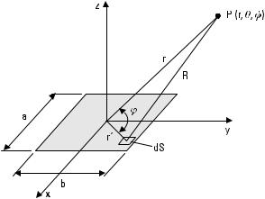
Figure 9.20 shows a rectangular radiating aperture, which is in the xy -plane and whose center is at the origin. The width of the aperture is a in the x -direction and b in the y -direction. The electric field Ex has a constant amplitude and phase over the whole aperture. The magnetic field is Hy = Ex /h. Thus, the aperture is like a part of a plane wave.
Far away from the aperture the field is obtained by integrating the field of the surface element, (9.35) and (9.36), over the aperture. Because the aperture field is constant, the integration simplifies to an integration of the phase term e −jkR, where the distance from the surface element to the point of observation P varies. Far from the aperture
R ≈ r − r ′ cos w |
(9.38) |
where r ′ is the distance of the surface element from the origin and w is the angle between the vectors r and r ′. The variable term r ′ cos w can be written as
Antennas |
227 |
Figure 9.20 Radiating aperture.
r ′ cos w = ur ? r ′
= (ux sin u cos f + uy sin u sin f + uz cos u ) ? (ux x ′ + uy y ′)
= x ′ sin u cos f + y ′ sin u sin f |
(9.39) |
where x ′ and y ′ are the coordinates of the surface element. Integration gives the u -component of the electric field:
b /2 a /2
Eu = |
|
|
jEx |
−jkr |
(1 + cos u ) cos f |
E |
E e |
jk (x ′ sin u cos f + y ′ sin u sin f ) |
dx ′ dy ′ |
||||||||||||||
|
|
|
|
e |
|
|
|
|
|
|
|||||||||||||
2lr |
|
|
|
|
|
|
|||||||||||||||||
|
|
|
|
|
|
|
|
|
|
|
|
|
|
−b /2 −a /2 |
|
|
|
||||||
|
|
|
|
|
|
|
|
|
|
|
|
3 |
sin S |
1 |
ka sin u cos fD |
4 |
|
||||||
= |
|
|
jabEx |
e |
−jkr |
(1 + cos u ) cos f |
2 |
|
|||||||||||||||
|
|
|
2l r |
|
|
|
1 |
|
|
|
|
||||||||||||
|
|
|
|
|
|
|
|
|
|
|
|
|
|
|
|
||||||||
|
|
|
|
|
|
|
|
|
|
|
|
|
|
|
|
|
ka sin u cos f |
|
|||||
|
|
|
|
|
|
|
|
|
|
|
|
|
|
|
|
2 |
|
||||||
|
|
|
|
3 |
sin S |
1 |
kb sin u sin fD |
4 |
|
|
|
|
|
|
|
|
|
|
|||||
|
? |
2 |
|
|
|
|
|
|
|
|
|
(9.40) |
|||||||||||
|
|
|
1 |
kb sin u sin f |
|
|
|
|
|
|
|
|
|
||||||||||
|
|
|
|
|
|
|
|
|
|
|
|
|
|
|
|
||||||||
|
|
|
|
|
|
2 |
|
|
|
|
|
|
|
|
|
|
|||||||
Correspondingly, the f -component is

228 Radio Engineering for Wireless Communication and Sensor Applications
|
|
|
|
|
|
|
|
|
|
|
3 |
sin S |
1 |
ka sin u cos fD |
4 |
|
|||
Ef = |
|
jabEx |
|
e |
−jkr |
(1 + cos u ) (−sin f) |
2 |
|
|||||||||||
|
|
2lr |
|
|
|
|
1 |
ka sin u cos f |
|
|
|||||||||
|
|
|
|
|
|
|
|
|
|
|
|
||||||||
|
|
|
|
sin S |
|
kb sin u sin f D |
|
2 |
|
|
|||||||||
|
|
|
3 |
1 |
4 |
|
|
|
|
|
|
|
|
||||||
|
? |
2 |
|
|
|
|
|
|
(9.41) |
||||||||||
|
|
|
|
|
|
|
|
|
|
|
|
|
|
||||||
|
|
|
1 |
kb sin u sin f |
|
|
|
|
|
|
|
||||||||
|
|
|
|
|
|
|
|
|
|
|
|
|
|||||||
|
|
|
|
2 |
|
|
|
|
|
|
|
|
|
||||||
In the E - |
|
or xz -plane (f = |
|
0°), the electric field has |
only |
the |
|||||||||||||
Eu -component, |
and in the H - |
or yz -plane |
|
(f = 90°), |
only |
the |
|||||||||||||
Ef -component.
If the aperture is large (a and b >> l ), the field is significant at small u angles only. Then cos u ≈ 1 and sin u ≈ u, and the normalized directional patterns in the E - and H -planes simplify to
|
| |
sin S |
1 |
kau D |
| |
|
|
|||||||||
En (u, f = 0°) = |
2 |
|
(9.42) |
|||||||||||||
|
|
|
1 |
kau |
|
|||||||||||
|
|
|
|
|
|
|||||||||||
|
| |
2 |
| |
|
||||||||||||
|
|
|
|
|
|
|
|
|
|
|
||||||
|
|
sin S |
1 |
kbu D |
|
|||||||||||
En (u, f = 90°) = |
|
2 |
(9.43) |
|||||||||||||
|
|
|
1 |
kbu |
|
|
||||||||||
|
|
|
|
|
|
|
||||||||||
|
|
2 |
|
|
|
|||||||||||
|
|
|
|
|
|
|
|
|
|
|
|
|||||
Figure 9.21 shows the directional pattern in the E -plane. It can be solved from (9.42) that the first null in the E -plane is at an angle of
u0 |
= |
l |
|
|
(9.44) |
||
a |
|||||||
|
|
|
|
||||
and the half-power beamwidth is |
|
|
|
|
|
|
|
u3dB |
≈ 0.89 |
l |
(9.45) |
||||
a |
|||||||
|
|
|
|
|
|
||
and the level of the first sidelobe is −13.3 dB.

|
|
|
|
|
|
Antennas |
229 |
|||||||||||||
|
|
|
|
|
|
|
|
|
|
|
|
|
|
|
|
|
|
|
|
|
|
|
|
|
|
|
|
|
|
|
|
|
|
|
|
|
|
|
|
|
|
|
|
|
|
|
|
|
|
|
|
|
|
|
|
|
|
|
|
|
|
|
|
|
|
|
|
|
|
|
|
|
|
|
|
|
|
|
|
|
|
|
|
|
|
|
|
|
|
|
|
|
|
|
|
|
|
|
|
|
|
|
|
|
|
|
|
|
|
|
|
|
|
|
|
|
|
|
|
|
|
|
|
|
|
|
|
|
|
|
|
|
|
|
|
|
|
|
|
|
|
|
|
|
|
|
|
|
|
|
|
|
|
|
|
|
|
|
|
|
|
|
|
|
|
|
|
|
|
|
|
|
|
|
|
|
|
|
|
|
|
|
|
|
|
|
|
|
|
|
|
|
|
|
|
|
|
|
|
|
|
|
|
|
|
|
|
|
|
Figure 9.21 Normalized directional pattern of a rectangular aperture.
The maximum power density produced by the rectangular aperture is
|
2h S |
l r |
D |
|
|
Smax = |
1 |
|
Ex ab |
2 |
(9.46) |
|
|
|
|
||
Because e−∞∞ sin2 x /x 2 dx = p , the average power density produced by a large aperture is
Sav = |
1 |
EES d V ≈ |
1 |
2p 2p |
(9.47) |
|||
|
|
Smax |
|
|
|
|||
4p |
4p |
ka |
kb |
|||||
|
|
4p |
|
|
|
|
|
|
The ratio of these power densities, the directivity, is
D = |
Smax |
= |
4p |
ab |
(9.48) |
|
|
||||
|
Sav l 2 |
|
|||
Assuming a lossless aperture (D = G ) and comparing (9.48) to (9.4), we
can see that the physical and effective areas are equal, that is, ab = A eff . The radiation pattern of an aperture antenna having an arbitrary shape,
amplitude distribution, and phase distribution is calculated using the same principle as above: The fields produced by the surface elements are summed at the point of observation.
If a rectangular aperture has a field distribution of a form f (x ) g ( y ), the normalized patterns in the xz - and yz -planes are those of the line sources

230 Radio Engineering for Wireless Communication and Sensor Applications
(one-dimensional apertures) having aperture distributions of f (x ) and g ( y ), respectively. The normalized pattern is the product of the normalized patterns in the xz - and yz -planes.
Table 9.1 shows properties of line sources having different amplitude distributions. The constant amplitude distribution gives the narrowest beam but the highest level of sidelobes. If the amplitude of the field decreases toward the edge of the aperture, the beamwidth increases, the gain decreases, and the sidelobe level decreases.
Earlier it was assumed that the phase of the aperture was constant. In practice, a quadratic phase distribution is usual. Then constant phase fronts are nearly spherical in the aperture. Figure 9.22 shows directional patterns for line sources having a constant amplitude but quadratic phase distribution. As the parameter D (phase difference between the center and edge in wavelengths) increases, gain decreases, sidelobes increase, and nulls get filled.
The properties of circular apertures are listed in Table 9.2 for different amplitude distributions (the phase is constant). If the aperture has a constant amplitude, the normalized directional pattern is
En (u ) = 2 | |
J1 S |
1 |
kD sin u D |
| |
|
||
2 |
(9.49) |
||||||
|
1 |
kD sin u |
|||||
2 |
|
||||||
|
|
|
|
|
|||
where D is the diameter of the aperture and J1 is the Bessel function of the first kind of order one.
Table 9.1
Properties of Line Sources
Amplitude |
|
|
|
|
Distribution |
Half-Power |
Level of First |
Position of |
|
in Aperture |
Beamwidth |
Sidelobe |
First Null |
|
|
|
|
|
|
Constant |
0.89l /a |
−13.3 |
dB |
l /a |
cos (p x /a ) |
1.19l /a |
−23.1 |
dB |
1.5l /a |
cos2(p x /a ) |
1.44l /a |
−31.5 |
dB |
2.0l /a |
1 − 0.5(2x /a )2 |
0.97l /a |
−17.1 |
dB |
1.14l /a |
Taylor, n = 3, |
|
|
|
|
edge −9 dB |
1.07l /a |
−25.0 dB |
— |
|
|
|
|
|
|

|
|
|
|
Antennas |
231 |
|||||||||
|
|
|
|
|
|
|
|
|
|
|
|
|
|
|
|
|
|
|
|
|
|
|
|
|
|
|
|
|
|
|
|
|
|
|
|
|
|
|
|
|
|
|
|
|
|
|
|
|
|
|
|
|
|
|
|
|
|
|
|
|
|
|
|
|
|
|
|
|
|
|
|
|
|
|
|
|
|
|
|
|
|
|
|
|
|
|
|
|
|
|
|
|
|
|
|
|
|
|
|
|
|
|
|
|
|
|
|
|
|
|
|
|
|
|
|
|
|
|
|
|
|
|
|
|
|
|
|
|
|
|
|
|
|
|
|
|
|
|
|
|
|
|
|
|
|
|
|
|
|
|
|
|
|
|
|
|
|
|
|
|
|
|
|
|
Figure 9.22 Directional pattern of a line source having a constant amplitude and quadratic phase distribution; D is the phase difference between the center and edge of the aperture in wavelengths.
Table 9.2
Properties of Circular Apertures
Amplitude |
|
|
|
|
Distribution |
Half-Power |
Level of First |
Position of |
|
in Aperture |
Beamwidth |
Sidelobe |
First Null |
|
|
|
|
|
|
Constant |
1.02l /D |
−17.6 dB |
1.22l /D |
|
1 − r 2 |
1.27l /D |
−24.6 |
dB |
1.63l /D |
(1 − r 2 )2 |
1.47l /D |
−30.6 |
dB |
2.03l /D |
0.5 + 0.5(1 − r 2 )2 |
1.16l /D |
−26.5 |
dB |
1.51l /D |
Taylor |
1.31l /D |
−40.0 |
dB |
— |
|
|
|
|
|