At frequencies that do not penetrate the ionosphere, that is, in the HF band and at lower frequencies, noise from electric discharge in the atmosphere (lightning) is dominant. The amount depends on the season and day, location, and frequency.

Noise from space dominates at frequencies from 20 MHz to 1 GHz. The Milky Way produces RF noise, which is at its maximum in the plane of the Milky Way and decreases as the direction goes away from this plane. The Milky Way noise also decreases as frequency increases. At all frequencies there is a 3K cosmic background radiation, which has its origin in the Big Bang, that is, it is a remnant of the birth of the universe.

Thermal noise due to the atmospheric attenuation is the dominating noise source above 1 GHz. It depends on the atmospheric humidity and elevation angle. The atmosphere can be considered as an attenuator at a physical temperature of about 270K.

Noise due to human activity may be considerable, especially near densely populated areas. In the VHF band and at lower frequencies, noise from the spark plugs of cars and power lines may be stronger than that from nature.

11.3 Modulation and Demodulation of Signals

Information to be transmitted in a radio system, such as voice or music, is first transformed to a low frequency, for example, an audio frequency, electric signal. This baseband signal cannot be directly transmitted through a radio channel, or at least that would be very inefficient. The signal is first fed into a modulator, which modulates some property (amplitude, frequency, phase) of a high-frequency carrier according to the baseband signal. The highfrequency signal obtained is then transmitted by a transmitting antenna. A receiving antenna receives the high-frequency signal and feeds it into a receiver. In the receiver the signal is often downconverted to an intermediate frequency and then demodulated, that is, the original baseband signal is detected; for example, in the case of voice radio, the original voice signal is recovered. In other words, with a modulator the information is attached into a carrier, and with a demodulator it is detached.

There are a number of different modulation schemes, which can be divided into analog and digital methods. Modulation is important not only in communication (radio broadcasting, radio links, mobile phone systems) but also in radar, radionavigation, and so on. Modulation is treated in many communication textbooks, for example, [8–10].

288 Radio Engineering for Wireless Communication and Sensor Applications

11.3.1 Analog Modulation

A sinusoidal waveform can be presented as

Information can be attached into this carrier by modulating one of its basic properties according to the baseband signal. Modulation methods are:

1.Amplitude modulation (AM): Information is attached to the carrier amplitude.

2.Frequency modulation (FM): Information is attached to the carrier frequency.

3.Phase modulation (PM): Information is attached to the carrier phase.

AM is in principle the simplest method, but it has high requirements, especially for the linearity of the transmitter. It is used in radio broadcasting in the LF, MF, and HF bands, and in TV broadcasting. FM is used, for example, in FM radio.

11.3.1.1 AM

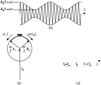
Let us consider a signal that is amplitude modulated by a sinusoidal signal at frequency f m :

Thus, the amplitude varies between values of A 0 (1 − m ) and A 0 (1 + m ). Factor m is the modulation index or modulation depth. The signal envelope follows the modulating signal as shown in Figure 11.9(a), if m < 1. The carrier frequency should be much higher than the modulating frequency. Equation (11.28) can be presented as

A (t ) = A 0 Fcos v 0 t + m2 cos (v 0 + vm ) t + m2 cos (v0 − vm ) tG (11.29)

The graphical interpretation of this equation is presented in Figure 11.9(b). A constant voltage phasor A 0 corresponds to the carrier frequency. Two voltage phasors with an amplitude of (m /2) A 0 rotate in opposite

Figure 11.9 Amplitude-modulated signal: (a) in time domain; (b) phasor presentation; and

(c) frequency spectrum.

directions at an angular frequency of vm . The resultant of these three voltage phasors gives the total voltage. The spectrum contains the components at frequencies f 0 , f 0 + f m , and f 0 − f m , as shown in Figure 11.9(c).

If the modulating baseband signal is more complicated, it can be considered as consisting of several sinusoidal components, which have a given amplitude and phase. The modulating signal has a given spectrum and each spectral component modulates the carrier independently.

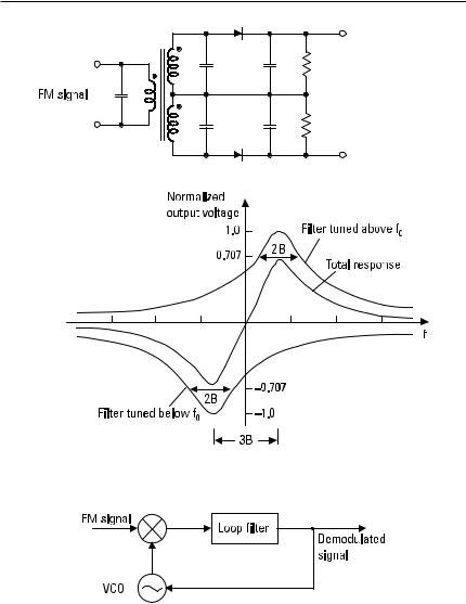
Figure 11.10 presents the spectrum of an AM signal when the modulating signal is distributed over a given frequency range. The AM is using lavishly both the power and frequency spectrum, because also the carrier not containing information is transmitted and one sideband is only a mirror image of the other. Transmitter power can be saved using DSB modulation, in which the carrier is suppressed, that is, it is not transmitted. This modulation scheme is also called double-sideband suppressed carrier (DSBSC) modulation. The frequency spectrum is saved by removing the other sideband, which leads to SSB modulation.

If the modulating signal contains frequency components near the zero frequency, use of SSB modulation becomes complicated, because it is difficult to separate the sidebands. Vestigial sideband (VSB) modulation is a compromise between SSB and DSB modulations. In VSB, one sideband is trans-

294 Radio Engineering for Wireless Communication and Sensor Applications

Figure 11.18 Spectrum of a frequency-modulated signal when the modulation index is m = 5.52.

spectrum looks like the AM spectrum, but the phases of the sidebands are different.

In theory the FM signal requires an infinite bandwidth. If we allow a given maximum distortion, we can limit the bandwidth. According to Carson’s rule the required bandwidth is [10]

11.3.1.5 Frequency Modulators and Demodulators

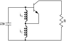
FM can be realized with a VCO. The output frequency of some oscillators can be controlled directly by changing the operation point of the nonlinear element. In other VCOs the frequency is controlled by voltage tuning the resonance frequency of the high-Q embedding circuit, which contains a voltage-dependent element such as a varactor.

Figure 11.19 shows a Hartley oscillator. The input network contains a varactor. The resonance frequency of the input resonator is

Let us assume that C changes sinusoidally an amount of DC around C0 and that the ratio DC /C 0 is small. Then