

24 |
POWER EXCEL WITH MR EXCEL |
|
|
|
SET UP EXCEL ICONS TO OPEN A SPECIFIC FILE ON STARTUP |
Problem: I routinely use the same five files in my job. I want a series of five icons on my Desktop so I can easily open these five files.
Strategy: You can use a startup switch in the shortcut. Excel offers startup switches to open a specific file, to open a file as read-only, to suppress the startup screen, or to specify an alternate default file location.
Follow these steps.
1. Open Windows Explorer using Win+M.
2. Browse to %ProgramFiles%\Microsoft Office\Office16\
3. If Windows Explorer is in full-screen mode, click the Restore Down button so you can see the desktop. 4. Scroll down to the Excel.exe entry. Right-click and drag it to the Desktop.
5. Choose Create Shortcuts Here from the menu that appears when you release the right mouse button. 6. On the Desktop, right-click the new Shortcut to Excel icon and choose Properties.
7. In the Properties dialog, choose the General tab.
8. Change the name in the top text box to something meaningful. If this icon will be used to open the
Sales file, for example, a short name like Sales would work.
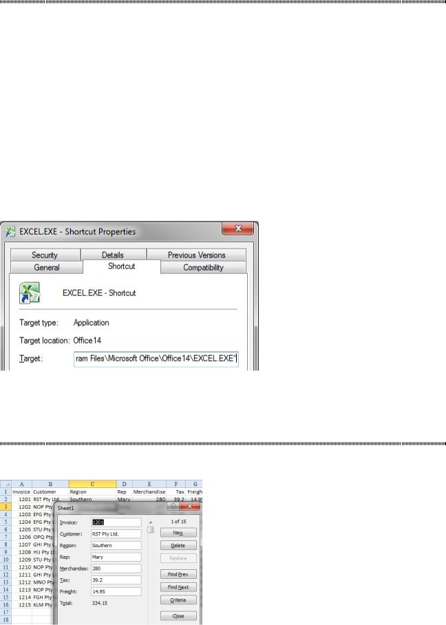
9. On the Shortcut tab, locate the Target field. As you can see below, this field contains the complete path and file name to EXCEL.EXE, with the path and file name enclosed in quotation marks. (The Target field is not big enough to display the entire path, so you must click in the field and press the End key in order to see the end of the entry.)
Figure 54 Use the End key to move to the end of the field.
10.After the final quote in the Target field, type a space and the path and file name. You can now click that icon to open the particular Excel file.
USE A MACRO TO CUSTOMIZE STARTUP
Problem: Every time I open a workbook, I would like to put the file in Data Form mode or invoke another Excel menu as the file opens.
Figure 55 The data form is increasingly difficult to find in Excel.
PART 1: THE EXCEL ENVIRONMENT |
25 |
|
|
Strategy: Startup switches can only do so many things. You will have to use a Workbook_Open macro in order to force Excel into Data Form mode. Follow these steps:
1. In Excel, type Alt+T followed by M and S.
2. Choose Disable All Macros with Notification. Click OK.
3. Open your workbook.
4. Press Alt+F11 to open the VBA Editor. Gotcha: The Microsoft Natural Multimedia keyboard does not support the use of Alt+function keys. You might have to type Alt+T followed by M and D.
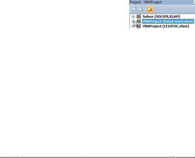
5. Press Ctrl+R to show the Project Explorer in the upper-left corner. You should see something that looks like VBAProject (Your BookName) in the Project Explorer.
|
Figure 56 Click the + to expand the project. |
1 |
6. |
If there is a + to the left of this entry, press the + to expand it. You will see a folder underneath, |
|
|
||
|
called Microsoft Excel Objects. If there is a + to the left of this entry, press the + to expand it, also. |
|
7. |
You will now see one entry for each worksheet, plus an entry called ThisWorkbook. |
|
Right-click ThisWorkbook and choose View Code from the context menu. |
|
|
8. |
Copy these three lines of code to the large white code window: |
|
Private Sub Workbook_Open() |
|
|
ActiveSheet.ShowDataForm |
|
|
End Sub |
|
|
9. |
Press Alt+Q to return to Excel. |
|
10.Select File, Save As, Excel Macro-Enabled Workbook. 11.Close the file.
12.Open the file. The information bar tells you that macros have been disabled. 13.Select Options, Enable This Content. The data form will open.
Alternate Strategy: To prevent Excel from automatically disabling macros, you can save the file in a trusted location. See “Use a Trusted Location to Prevent Excel’s Constant Warnings” earlier in this sec- tion.
Gotcha: The data form used to be an option on the Excel 2003 Data menu. It is hidden in Excel today. To invoke this command, you can either press Alt+D+O or add the command to your Quick Access toolbar.
Additional Details: The simple Workbook_Open macro invokes a Menu command. It is possible to build highly complex macros that would control literally anything. For a primer on macros, consult VBA and Macros for Microsoft Excel 2013 from Que Publishing.
CONTROL SETTINGS FOR EVERY NEW WORKBOOK AND WORKSHEET
Problem: Every time I start a new workbook or insert a new worksheet, I always make the same custom- izations, such as setting print scaling to fit to one page wide, setting certain margins, adding a “Page 1 of n” footer to the worksheet, making the heading row bold, and so forth. How can I have these settings applied to every new workbook or worksheet?
Strategy: Two files control the defaults for new workbooks and inserted worksheets. You can easily cus- tomize a blank workbook to contain your favorite settings and then save the file as book.xltx and sheet. xltx. Then, any time you either click Ctrl+N for a new workbook or insert a worksheet, the new book or sheet will inherit the settings from these files. Follow these steps to create book.xltx:
1. In Excel, open a new blank workbook with Ctrl+N.
2. Customize the workbook as you like. Feel free to make adjustments to any of the following: ●● Page layout settings
●● The print area ●● Cell styles
●● Formatting commands on the Home tab ●● Data, Validation settings
●● The number and type of sheets in the workbook ●● The window view options from the View tab
26 |
POWER EXCEL WITH MR EXCEL |
|
|
3.Decide where you want to save the file. This can be either in the XLStart folder (generally C:\Pro- gram Files\Microsoft Office\Officenn\XLStart) or in the alternate startup folder. (See “Have Excel Always Open Certain Workbooks”.)
4.Select File, Save As, Other Formats.
5.In the Save As dialog, open the Save as Type dropdown and choose Excel Template (*.xltx).
6.Browse to the XLStart folder you specified in step 3.
7.Save the file as book.xltx.
Results: All subsequent new workbooks created with Ctrl+N will inherit the settings from the book.xltx file.
Gotcha: Excel 1 through Excel 2003 had a “New” icon on the Standard toolbar and a “New…” icon on the File menu. While these icons sound similar, they are very different. The regular “New” icon will create a new workbook based on book.xltx. The “New…” icon leads to a panel where you can select a template from Office Online. This trick will not work with the File, New command in Excel 2010. You have to use Ctrl+N or add the old “New” icon to the QAT or ribbon. The problem is worse in Excel 2013, where the Blank Workbook tile offered on the Start Screen is equivalent to “New…” and will not load Book.xltx.
Additional Details: You should also set up a workbook with one worksheet and save this workbook as sheet.xltx. All inserted worksheets will inherit the settings from this file.
Additional Details: If you regularly create macros, save the files with the .xltm extension instead.
EXCEL SAYS I HAVE LINKS, BUT I CAN NOT FIND THEM
Problem: When I open a workbook, Excel tells me there are external links in the file. Where are they?
Strategy: Use Ctrl+F to open the Find dialog. Open the Options>> button and change the Within drop- down from Sheet to Workbook. Search for a left square bracket. If the links are in a formula in a cell, this technique will find the link. If nothing is found, then go to Formulas, Name Manager. Links are often lurk- ing in out-of-use named ranges. I’ve also seen links hiding in the Data, Consolidate dialog box.
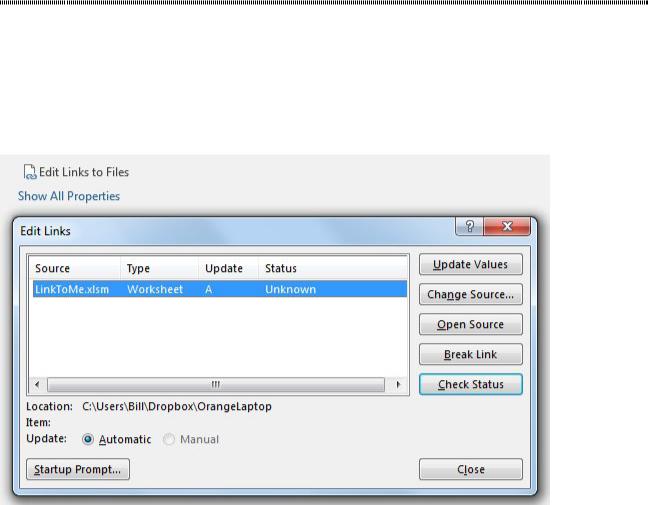
If you want to break the links or change the source to a new location, open the File menu. On the right side of the screen, look for Related Documents and click the Edit Links to Files hyperlink.
Figure 57 Break links or change the source file.
PART 1: THE EXCEL ENVIRONMENT |
27 |
|
|
AUTOMATICALLY MOVE THE CELL POINTER AFTER ENTER
Problem: If I type a number and then press a direction arrow key, Excel will enter the number and move the cell pointer in the direction of the arrow key. However, if I am using the numeric keypad, it is much more convenient to use the Enter key on the numeric keypad than to use the arrow keys. By default, Excel will move the cell pointer down one cell when I press Enter. Is there a way to have Excel automatically move the cell pointer to the next cell to the right after each entry?
Strategy: You can select File, Options. On the Advanced tab of the Excel Options dialog, you select the first setting, “After Pressing Enter, Move Selection Direction,” and choose Right from its dropdown.
Results: The cursor will automatically move one cell to the right every time you press the Enter key.
Additional Details: Override this setting by pressing Ctrl+Enter. The cell pointer will stay in the current cell.
RETURN TO THE FIRST COLUMN AFTER TYPING THE LAST COLUMN |
1 |
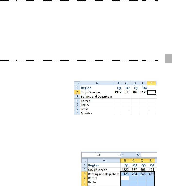
Problem: I learned in “Automatically Move the Cell Pointer in a Direction After Entering a Number” how to set up the cell pointer to move right after I press Enter. This works great. I just typed figures for Q1, Q2, Q3, and Q4 (see below). So I can quickly enter all four quarters, is there any way to make Excel jump to cell B3 after I type in cell E2?
Figure 58 Can Excel jump to the first column in the next row?
Strategy: Yes! Here’s what you do:
1. Set up Excel to move right as described in the previous topic.
2. Select the range before you start typing the data. For example, in the figure above, you might select
B3:E99. Although you have selected a rectangular range, B3 is the active cell. 3. Type 123 and press Enter. Excel will move to B4.
4. Repeat this to fill in the numbers for Q2, Q3, and Q4. When you press Enter in cell E3, Excel will move to B4.
Figure 59 Excel will jump to B4 from E3
Alternate Strategy: There is another way to handle this situation, although it’s not as straightforward as the method just described. Whereas the method just described requires you to use Right as the Move
Selection Direction, this strategy requires that setting to be set to Down:
1. Select File, Options, Advanced. Open the dropdown for After Pressing Enter, Move Selection Direc- tion, and choose Down. Click OK.
2. Select cell B5. Type a value and press Tab. Excel will jump to C5. 3. Type a value for Q2 and press Tab. Excel will jump to D5.
4. Type a value for Q3 and press Tab. Excel will jump to E5.
5. Type a value for Q4 and press Enter. Excel will jump back to cell B6!