

PART 2: CALCULATING WITH EXCEL |
131 |
|
|
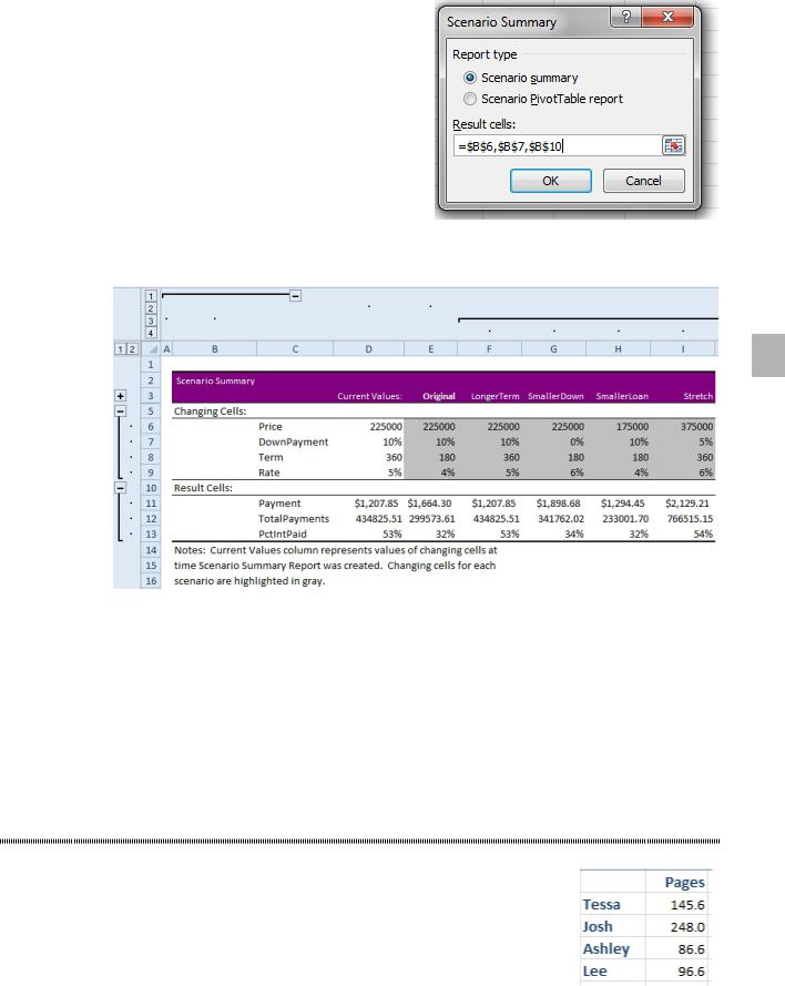
11.To see a comparison of all scenarios, click Summary.
12.In the Scenario Summary dialog, specify the output cells to include in the report.
Figure 324 Specify output cells.
13.A new worksheet is inserted. It will contain a column for each scenario. Input cells appear in grey. Output cells appear below.
2
Figure 325 The summary report compares the scenarios.
Additional Details: Group and Outline symbols appear around the report. Clicking the minus symbol above column C will hide the notes in rows 14:16 and produces a cleaner report. Clicking the plus symbol to the left of row 3 will reveal the description that you entered for each scenario. Minus symbols next to row 5 or 10 hide the input or output section of the report. The minus symbol above the final column hides all of the scenarios, leaving only the current values.
The scenario manager is relatively difficult to use because you must build each scenario by typing the values into a dialog. I wrote the MrExcel Monte Carlo Analysis add-in to allow you to specify the scenarios by saying that Price should go from 175,000 to 325,000 in $25,000 increments. Using this method, you can build dozens or hundreds of scenarios very quickly.
RANK SCORES
Problem: I have four writers working on a project. Each week, I need to report how many pages they have written toward their goal. I want to add a formula to rank them in high-to-low order.
Figure 326 Rank the scores.
132 |
POWER EXCEL WITH MR EXCEL |
|
|
Figure 327 Assign a rank.
PART 2: CALCULATING WITH EXCEL |
133 |
|
|
1. |
Figure 329 The table in rows 8:11 sorts the original data. |
|
|
Set up a new table with numbers 1 through 4. |
|
||
2. |
The formula in B8:B11 is =VLOOKUP($A8,$A$2:$C$5,2,FALSE). |
|
|
3. |
The formula in C8:C11 is =VLOOKUP($A8,$A$2:$C$5,3,FALSE). |
|
|
After using a RANK function to assign rank values to a list, you can use a second table with the numbers |
|
||
2 |
|||
1 through n and a series of VLOOKUP formulas in order to return a sorted list of the data. |
|||
|
|
|
|
ROUND NUMBERS
Problem: My formula is producing results with many decimal places. I need to round to the nearest cent or nearest dollar or even to the nearest hundred dollars.
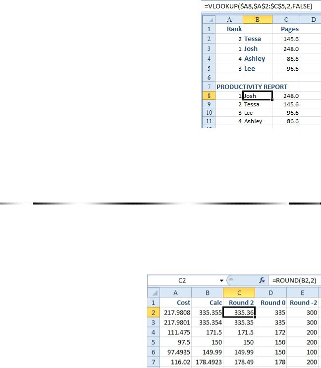
Strategy: Use the versatile ROUND function. The function requires a number to be rounded then a precision value. If you use =ROUND(B2,2) you will round numbers to the nearest penny. If you use =ROUND(B2,0) you will round to the nearest dollar. The precision argument can be negative to indicate that you want to round to the left of the decimal point. If you use =ROUND(B2,-2) you will round to the nearest hundred dollars.
Figure 330 Round to the nearest penny, dollar, or hundred.
ROUND can use any number as the precision argument. Although the figure above shows 2, 0, and -2, you could carry this logic forward. To round to the nearest million, use a precision of -6. To round to the nearest thousandth, use a precision of 3.
Additional Details: If you always want to round up or round down, use ROUNDUP or ROUNDDOWN functions. They work just like ROUND, requiring the number to round and the precision. Note that ROUNDUP will round away from zero. This makes sense for positive numbers, the ROUNDUP(1.01,0) will be 2. For negative numbers, the ROUNDUP(-1.01,0) will be -2. This is tricky, since -2 is actually lower than -1.01. If you want -1.01 to round to -1, then use =CEILING(1.01,1).

134 |
POWER EXCEL WITH MR EXCEL |
|
|
|
ROUND TO THE NEAREST $0.05 WITH MROUND |
Problem: I know I can use the ROUND function to round to the nearest dollar or penny. How do I round to the nearest nickel or quarter?
Strategy: You can use the MROUND func- tion. This function will round a number to the nearest multiple of the second argument. To round to the nearest nickel, use
=MROUND(B2,0.05). To round to the near- est quarter, you use =MROUND(B2,0.25).
Figure 331 Round to the nearest 0.05.
Gotcha: Both arguments in the MROUND function must have the same sign. This can be difficult when you have a mixture of positive and negative values. The SIGN function will return either a 1 or -1, based on the sign of a number. If there is a possibility that the first argument might be negative, you can multiply the second argument by SIGN of the first argument. =MROUND(B2,0.05*SIGN(B2))
ROUND PRICES TO THE NEXT HIGHEST $5
Problem: I handle pricing for a company, and I have a spreadsheet that shows my cost per SKU. My manager tells me to take the current manufacturing cost for each item, multiply by 2, add $3, and then round up to the next highest multiple of 5.
Figure 332 38.9615 doesn’t make a nice price.
Strategy: After doing the math to get a preliminary price, you can use the CEILING function. This function takes one number and the number to round up to. For example,
=CEILING(421,5) will result in 425. Note that with CEIL- ING, the answer is always higher than the original number.
Additional Details: Excel also has a FLOOR function. With the FLOOR function, the number would be rounded down to the nearest multiple of 5.
Figure 333 Use CEILING to round up to a multiple.
ROUND 0.5 TOWARDS EVEN PER ASTM-E29
Problem: Excel always rounds 0.5 up to the next integer. The latest best practice in rounding says to round 0.5 towards the even number.
Back in school, you probably learned to round 0.5 up to the next highest number. In a large data set, this rule is leading to the data set being slightly skewed higher. The guidance published by the ASTM in their rule E29 says that numbers ending in 0.5 should round towards the even number. Theoretically, half the time the number rounds up and half the time the number rounds down, cancelling out the skew.
Strategy: Use =IF(MOD(A2,1)=0.5,MROUND(A2,2),ROUND(A2,0)) instead of ROUND(A2,2).