

8 |
POWER EXCEL WITH MR EXCEL |
|
|
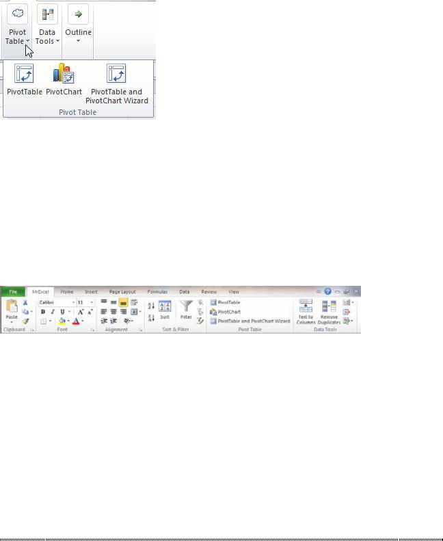
Figure 16 The icon from Figure 13 shows with a smaller window size.
Note back in Figure 9 that the Sort icon appears as a large icon with a caption and that the AZ and ZA icons appear as small icons without a caption. How can you specify that the pivot table icon should be large and the pivot chart and wizard icons should be small? You can’t. At least not with the Excel interface.
If you want to start writing some XML and VBA, you can gain control over the size and images used in the ribbon. For an excellent book on this daunting task, look for RibbonX: Customizing the Office 2007 Ribbon by Robert Martin, Ken Puls and Teresa Hennig. Or, check out the Ribbon Commander utility described at http://mrx.cl/2dbS4Js.
I find that I spend most of my time on either the Home or the Data tab. If I could combine the left side of the Home tab with the right side of the Data tab, plus pivot tables, I would probably be able to spend all my time on one tab.
This figure shows a new MrExcel tab that reuses groups from other ribbon tabs to build a new tab.
Figure 17 The MrExcel tab is a custom tab with my favorite groups.
The general steps for creating a new ribbon tab are as follows: 1. Right-click the Ribbon and choose Customize the Ribbon. 2. Click New Tab at the bottom right of the dialog.
3. Click Rename and give the tab a name.
4. Use the Up and Down buttons at the right side of the dialog to move the new tab into the proper location.
5. From the left dropdown, choose Main Tabs.
6. In the left dropdown, expand an existing tab and find an existing group that you want to add to your new tab. Click that group and click Add.
7. Repeat step 6 to add additional groups.
8. You can reuse a custom group that you created previously. In the left dropdown, choose Custom Tabs and Groups. You can move the Pivot Table (Custom) tab created earlier in this chapter onto your new ribbon tab.
9. Click OK to finish customizing the ribbon tab.
GO WIDE
Problem: My ribbon looks different than my co-workers.
Strategy: Invest in a wide-screen monitor. The Excel experience dramatically improves at a 1440x900 or 1920x1080 resolution.
When you reduce the size of the Excel window, Excel automatically starts consolidating ribbon options into smaller icons and then groups. The next four figures show details of the Home tab of the ribbon at different sizes.
PART 1: THE EXCEL ENVIRONMENT |
9 |
|
|
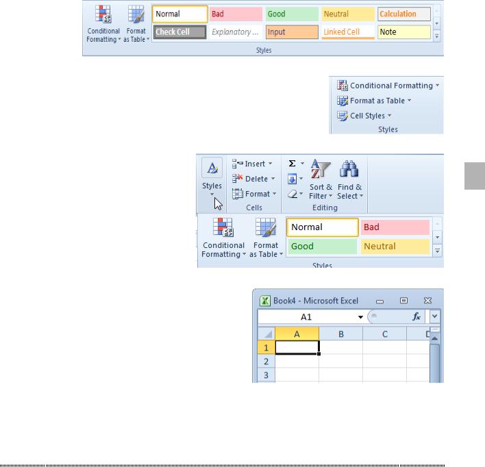
Figure 18 At 1920 wide, five columns of the gallery are shown
Figure 19 At a smaller screen, the cell styles gallery is a dropdown.
1
Figure 20 Eventually, the entire Styles group becomes a dropdown..
Figure 21 If the Excel window is too small, the Ribbon disappears.
If you are the go-to person for solving Excel problems and you are helping a co-worker over the phone without using GoToMeeting, there will be some frustration as you tell them to look for the Bad, Good, Neutral tiles and they can only see a Styles dropdown.
MINIMIZE THE RIBBON TO FREE UP A FEW MORE ROWS
Problem: The ribbon is taking up a lot of real estate at the top of my screen. It distracts me. I spend 99% of my Excel time in the grid, so I don’t need to see the ribbon all the time.
Strategy: You can minimize the ribbon, reducing it to a simple line of Home, Insert, Page Layout, For- mulas, and so on.
To minimize the ribbon, you can either press Ctrl+F1 or right-click anywhere on the ribbon and then choose Minimize the Ribbon. You can also use the carat (^) icon at the right edge of the ribbon.
Additional Details: When you either click a ribbon tab with the mouse or use an Excel shortcut key, the ribbon will temporarily reappear. When you select the command from the ribbon, it will minimize again.
Double-click any ribbon tab to permanently exit minimized mode. Or, open any ribbon tab and then use the thumbtack icon on the right edge of the ribbon.
10 |
POWER EXCEL WITH MR EXCEL |
|
|
|
USE A WHEEL MOUSE TO SCROLL THROUGH THE RIBBON TABS |
If you point your mouse at the ribbon and scroll the wheel, you will quickly move from Home to Insert to
Page Layout and so on.
WHY DO THE CHARTING RIBBON TABS KEEP DISAPPEARING?
Occasionally, new tabs will appear on the right side of the ribbon. These tabs appear when the current selection includes SmartArt graphics, charts, drawings, pictures, pivot tables, pivot charts, worksheet headers, tables, ink, or when you are in the legacy Print Preview mode.
These new tabs will stay visible as long as the object stays selected. If you click outside of your pivot table or chart, the tabs will disappear. If you are looking at an object and cannot find the tools necessary to edit the object, click the object to bring the tools back.
USE DIALOG LAUNCHERS FOR MORE CHOICES
Problem: It seems like there should be more choices than what is showing on the ribbon. Where is Center
Horizontally in the ribbon?
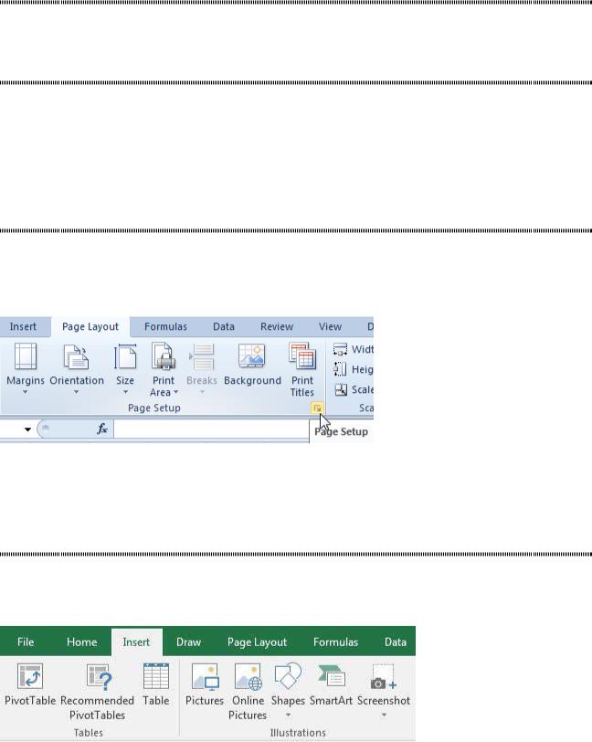
Strategy: Many groups in the ribbon contain a tiny icons called dialog launchers. You can click an icon to open a dialog with more choices. This figure shows an example of a dialog launcher.
Figure 22 Take me back to the old dialog.
Additional Details: It is difficult to describe the dialog launcher icon. If you enlarge the icon, you can see that it looks like the top-left corner of a square with an arrow pointing down and to the right. I am sure there is some artistic rationale why these pixels mean “launch the full dialog ,” but I can’t figure it out.
ICON, DROPDOWNS, AND HYBRIDS
Problem: The ribbon introduces several new types of controls.
In this figure, the Table and Pictures icon will invoke a command. The Shapes and Screenshot icons are dropdowns that lead to a flyout menu.
Figure 23 A mix of dropdowns, icons, and hybrids.
PART 1: THE EXCEL ENVIRONMENT |
11 |
|
|
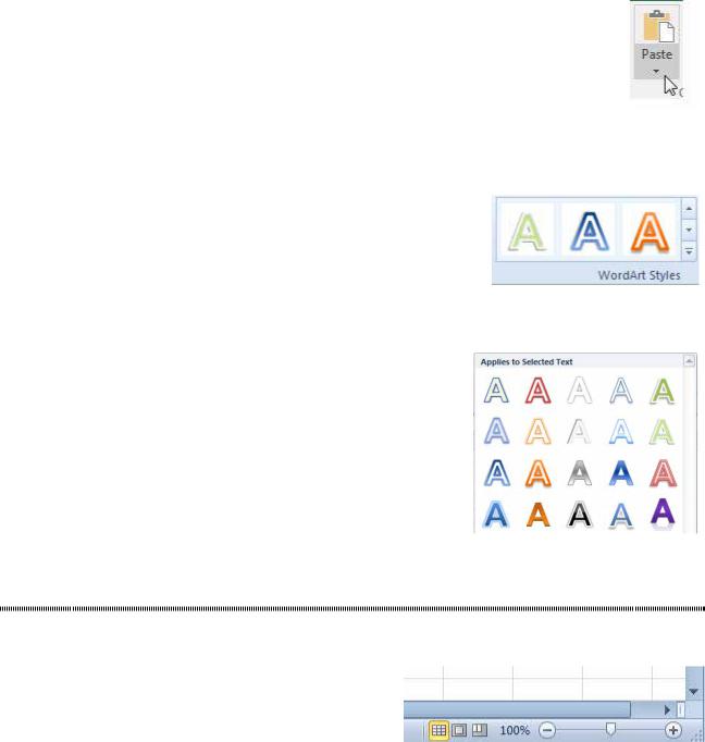
However, the Paste icon is actually two icons. The top half will do a default Paste. The bottom half leads to a flyout. You can’t really tell which icons are a hybrid of icon and dropdown until you hover over the icon with your mouse.
Figure 24 When you hover, a horizontal line divides the icon.
The other new type of control in the ribbon is a gallery with three |
|
|
|
arrows at the right side. The first and second arrows in the gallery |
|
|
|
will scroll through choices one row at a time. |
|
|
|
If you click the bottom arrow, the gallery will fly open to reveal all |
|
|
|
|
1 |
||
of the choices. |
|
||
Figure 25 Galleries have three ar- |
|
||
|
|
|
|
|
|
|
|
|
|
rows on the right edge. |
|
Additional Details: Several icons have an upper |
|
|
|
(icon) half and a lower (dropdown) half: |
|
|
|
●● |
Paste on the Home tab |
|
|
●● |
Insert on the Home tab |
|
|
●● |
Delete on the Home tab |
|
|
●● |
Bring Forward on the Page Layout tab |
|
|
●● |
Send Backward on the Page Layout tab |
|
|
●● |
AutoSum on the Formulas tab |
|
|
●● |
Data Validation on the Data tab |
|
|
●● |
Macros on the View tab |
|
|
Figure 26 Use bottom arrow to open the gallery.
ZOOM IS AT THE BOTTOM
Problem: Starting in Excel 2007, all commands in Office are supposed to be at the top of the screen. Don’t miss the View and Zoom commands at the bottom right of the window.
Figure 27 Control view and zoom in lower right.
Strategy: The icons in the lower-right corner of the screen control the zoom and switch between Normal view, Page Break Preview, and Page Layout view.
The zoom slider gives you one-click access to change the zoom from 10% up to 400%. This is easier to use than the old Zoom dropdown on the Standard toolbar. You just click the + icon at the right to increase the zoom in 10% increments. You click the, icon at the left to decrease the zoom in 10% increments, or you can simply drag the zoom slider to any spot along the continuum. To access the legacy Zoom dialog, click on the digits in the zoom percentage.
As in past versions of Excel, the quickest way to zoom in Excel is to use the wheel mouse. You hold down the Ctrl key while you scroll the wheel on your mouse forward to zoom in or backward to zoom out.
At a 400% zoom, you can get an ultra-close look at the detail of Excel’s High-Low-Close stock chart to see that they really don’t draw the left-facing Open symbol.