Figure 255 COUNTA returns the expected result.

Additional Details: COUNTA will not count blank cells. You use COUNTBLANK to return the number of empty cells in a range.

TOTAL THE RED CELLS

Figure 256 Total the red cells.

Strategy: Use the new filter by color to show only the red cells. Right-click on a red cell and choose Filter,

Filter by Cell Color.

Figure 257 Choose to filter by cell color.

Only the red cells will be shown. After applying the filter, go to the first visible blank cell below the data and press the AutoSum button or Alt+Equals. When applied to a filtered dataset, the AutoSum button switches from the SUM function to the SUBTOTAL function. This function will sum only the visible cells, providing a sum of the red cells.

Figure 258 AutoSum uses SUBTOTAL now.

Additional Details: This feature will work even if the red has been applied by conditional formatting.

Gotcha: When you clear the filter to show all cells, the formula will include the non-red cells. If you need a formula to add the red cells while displaying the other cells, you would have to use a User Defined Func- tion in the Excel VBA language. Watch this YouTube video: http://mrx.cl/sumredmacro for details.

AUTOMATICALLY NUMBER A LIST OF EMPLOYEES

Problem: I work in human resources, and I have a list of employees, separated by department. I have a numeric sequence in column A and the employees’ names in column B. Every time the company hires or fires an employee, I have to manually renumber all the employees. How can I make this job easier?

Figure 259 Numbering the employees manually is an HR nightmare.

Strategy: You can replace the numbers in column A with a formula that will count the entries in column

B. The formula should count from the current row all the way up to row 1.

The COUNT function will not work because it only counts numeric entries. You need to use the COUNTA function and keep in mind the following points:

●● The range that should be counted should extend from B1 to the current row. ●● The notation to always use B1 is B$1.

Here’s what you do:

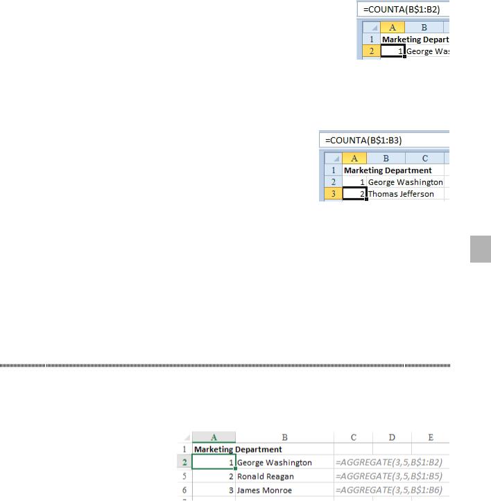
1. Enter the formula =COUNTA(B$1:B2) in cell A2.

Figure 260 Count from B1 to the current row.

When you copy this formula down a row, the range that is counted will extend from B1 to B3. This is because the B2 portion of the formula is a relative reference that is allowed to change as the formula is copied. The dollar sign in the B$1 reference tells Excel that when you copy the formula, it should always refer to row 1.

Figure 261 The range now extends from B1 to B3.

The range now extends from B1 to B3.

2. Copy the formula down to all the names in your list. They will be numbered just as when you typed

in the names in manually. 2

Results: When an employee leaves the company, you can simply delete the row, and all of the later rows will be renumbered. When you hire a new person, you can insert a blank row, enter the new hire’s name, and then copy any formula from another cell in A to the new row.

While this is a specific example, the concept of using a range as an argument where only one portion of the range contains an absolute reference is a common solution to keeping a running total of all cells above the current row.

AUTOMATICALLY NUMBER THE VISIBLE ROWS

Problem: What if you don’t delete the past employees, but you hide the rows? The newer AGGREGATE function can ignore hidden rows.

In the figure below, the first argument of 3 tells Excel to use the COUNTA function. The second argument of 5 tells Excel to ignore hidden rows.

Figure 262 AGGREGATE can ignore errors, other subtotals, or hidden rows.

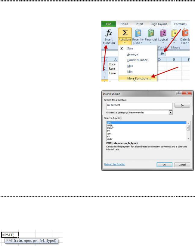
Problem: There are hundreds of functions available in Excel. I know that I want to find a function to cal- culate a car payment, but I have no clue which function might do this.

Strategy: To find a function, you can click the Insert Function (fx) button. This button is always avail- able to the left of the formula bar, and it appears 12 additional times in Excel, mostly on the Formulas tab. This figure shows three instances of the fx but- ton. You can click this button to bring up the Insert

Function dialog.

Figure 263 Three of the 13 fx icons.

By default, the Insert Function dialog lists the most recently used functions. All of Excel’s functions are categorized into these categories: Financial, Date & Time, Math & Trig, Statistical, Lookup & Reference,

Database, Text, Logical, Information, Cube, and

Engineering. It can be difficult to correctly guess the category. SUM is a Math & Trig function, yet AVERAGE is a Statistical function. Rather than browse each category, you can type a few words in the search box and click Go. Excel will show you the relevant functions to choose from.

Figure 264 Search for a function.

GET HELP ON ANY FUNCTION WHILE ENTERING A FORMULA

Problem: There are hundreds of functions available in Excel. Sometimes I remember that I need to use a particular function, but I cannot remember the sequence of the arguments in the function.

Strategy: If you type the equal sign followed by the function and the opening parenthesis, a ToolTip will appear reminding you of the order of the arguments. Any arguments in square brackets are optional. The argument in bold is the argument you need to type next.

Figure 265 The ToolTip lists the arguments.

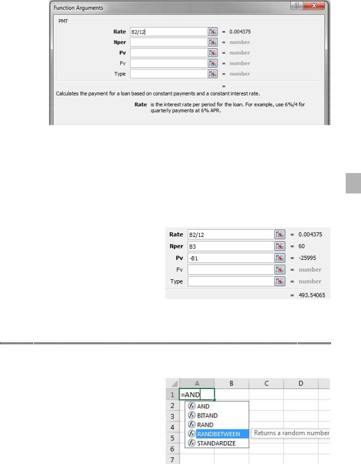
Alternate Strategy: If you need more help than the ToolTip’s abbreviations (for example, pmt, pv) pro- vide, you can use the Function Arguments dialog. To do so, you type the equals sign followed by the function name and the opening parenthesis, and then press Ctrl+A to display the Function Arguments dialog box.