

- •1. INTRODUCTION
- •1.1 BASIC TERMINOLOGY
- •1.2 EXAMPLE SYSTEM
- •1.3 SUMMARY
- •1.4 PRACTICE PROBLEMS
- •2. TRANSLATION
- •2.1 INTRODUCTION
- •2.2 MODELING
- •2.2.1 Free Body Diagrams
- •2.2.2 Mass and Inertia
- •2.2.3 Gravity and Other Fields
- •2.2.4 Springs
- •2.2.5 Damping and Drag
- •2.2.6 Cables And Pulleys
- •2.2.7 Friction
- •2.2.8 Contact Points And Joints
- •2.3 SYSTEM EXAMPLES
- •2.4 OTHER TOPICS
- •2.5 SUMMARY
- •2.6 PRACTICE PROBLEMS
- •2.7 PRACTICE PROBLEM SOLUTIONS
- •2.8 ASSIGNMENT PROBLEMS
- •3. ANALYSIS OF DIFFERENTIAL EQUATIONS
- •3.1 INTRODUCTION
- •3.2 EXPLICIT SOLUTIONS
- •3.3 RESPONSES
- •3.3.1 First-order
- •3.3.2 Second-order
- •3.3.3 Other Responses
- •3.4 RESPONSE ANALYSIS
- •3.5 NON-LINEAR SYSTEMS
- •3.5.1 Non-Linear Differential Equations
- •3.5.2 Non-Linear Equation Terms
- •3.5.3 Changing Systems
- •3.6 CASE STUDY
- •3.7 SUMMARY
- •3.8 PRACTICE PROBLEMS
- •3.9 PRACTICE PROBLEM SOLUTIONS
- •3.10 ASSIGNMENT PROBLEMS
- •4. NUMERICAL ANALYSIS
- •4.1 INTRODUCTION
- •4.2 THE GENERAL METHOD
- •4.2.1 State Variable Form
- •4.3 NUMERICAL INTEGRATION
- •4.3.1 Numerical Integration With Tools
- •4.3.2 Numerical Integration
- •4.3.3 Taylor Series
- •4.3.4 Runge-Kutta Integration
- •4.4 SYSTEM RESPONSE
- •4.4.1 Steady-State Response
- •4.5 DIFFERENTIATION AND INTEGRATION OF EXPERIMENTAL DATA
- •4.6 ADVANCED TOPICS
- •4.6.1 Switching Functions
- •4.6.2 Interpolating Tabular Data
- •4.6.3 Modeling Functions with Splines
- •4.6.4 Non-Linear Elements
- •4.7 CASE STUDY
- •4.8 SUMMARY
- •4.9 PRACTICE PROBLEMS
- •4.10 PRACTICE PROBLEM SOLUTIONS
- •4.11 ASSIGNMENT PROBLEMS
- •5. ROTATION
- •5.1 INTRODUCTION
- •5.2 MODELING
- •5.2.1 Inertia
- •5.2.2 Springs
- •5.2.3 Damping
- •5.2.4 Levers
- •5.2.5 Gears and Belts
- •5.2.6 Friction
- •5.2.7 Permanent Magnet Electric Motors
- •5.3 OTHER TOPICS
- •5.4 DESIGN CASE
- •5.5 SUMMARY
- •5.6 PRACTICE PROBLEMS
- •5.7 PRACTICE PROBLEM SOLUTIONS
- •5.8 ASSIGNMENT PROBLEMS
- •6. INPUT-OUTPUT EQUATIONS
- •6.1 INTRODUCTION
- •6.2 THE DIFFERENTIAL OPERATOR
- •6.3 INPUT-OUTPUT EQUATIONS
- •6.3.1 Converting Input-Output Equations to State Equations
- •6.3.2 Integrating Input-Output Equations
- •6.4 DESIGN CASE
- •6.5 SUMMARY
- •6.6 PRACTICE PROBLEMS
- •6.7 PRACTICE PROBLEM SOLUTIONS
- •6.8 ASSGINMENT PROBLEMS
- •6.9 REFERENCES
- •7. ELECTRICAL SYSTEMS
- •7.1 INTRODUCTION
- •7.2 MODELING
- •7.2.1 Resistors
- •7.2.2 Voltage and Current Sources
- •7.2.3 Capacitors
- •7.2.4 Inductors
- •7.2.5 Op-Amps
- •7.3 IMPEDANCE
- •7.4 EXAMPLE SYSTEMS
- •7.5 ELECTROMECHANICAL SYSTEMS - MOTORS
- •7.5.1 Permanent Magnet DC Motors
- •7.5.2 Induction Motors
- •7.5.3 Brushless Servo Motors
- •7.6 FILTERS
- •7.7 OTHER TOPICS
- •7.8 SUMMARY
- •7.9 PRACTICE PROBLEMS
- •7.10 PRACTICE PROBLEM SOLUTIONS
- •7.11 ASSIGNMENT PROBLEMS
- •8. FEEDBACK CONTROL SYSTEMS
- •8.1 INTRODUCTION
- •8.2 TRANSFER FUNCTIONS
- •8.3 CONTROL SYSTEMS
- •8.3.1 PID Control Systems
- •8.3.2 Manipulating Block Diagrams
- •8.3.3 A Motor Control System Example
- •8.3.4 System Error
- •8.3.5 Controller Transfer Functions
- •8.3.6 Feedforward Controllers
- •8.3.7 State Equation Based Systems
- •8.3.8 Cascade Controllers
- •8.4 SUMMARY
- •8.5 PRACTICE PROBLEMS
- •8.6 PRACTICE PROBLEM SOLUTIONS
- •8.7 ASSIGNMENT PROBLEMS
- •9. PHASOR ANALYSIS
- •9.1 INTRODUCTION
- •9.2 PHASORS FOR STEADY-STATE ANALYSIS
- •9.3 VIBRATIONS
- •9.4 SUMMARY
- •9.5 PRACTICE PROBLEMS
- •9.6 PRACTICE PROBLEM SOLUTIONS
- •9.7 ASSIGNMENT PROBLEMS
- •10. BODE PLOTS
- •10.1 INTRODUCTION
- •10.2 BODE PLOTS
- •10.3 SIGNAL SPECTRUMS
- •10.4 SUMMARY
- •10.5 PRACTICE PROBLEMS
- •10.6 PRACTICE PROBLEM SOLUTIONS
- •10.7 ASSIGNMENT PROBLEMS
- •10.8 LOG SCALE GRAPH PAPER
- •11. ROOT LOCUS ANALYSIS
- •11.1 INTRODUCTION
- •11.2 ROOT-LOCUS ANALYSIS
- •11.3 SUMMARY
- •11.4 PRACTICE PROBLEMS
- •11.5 PRACTICE PROBLEM SOLUTIONS
- •11.6 ASSIGNMENT PROBLEMS
- •12. NONLINEAR SYSTEMS
- •12.1 INTRODUCTION
- •12.2 SOURCES OF NONLINEARITY
- •12.3.1 Time Variant
- •12.3.2 Switching
- •12.3.3 Deadband
- •12.3.4 Saturation and Clipping
- •12.3.5 Hysteresis and Slip
- •12.3.6 Delays and Lags
- •12.4 SUMMARY
- •12.5 PRACTICE PROBLEMS
- •12.6 PRACTICE PROBLEM SOLUTIONS
- •12.7 ASIGNMENT PROBLEMS
- •13. ANALOG INPUTS AND OUTPUTS
- •13.1 INTRODUCTION
- •13.2 ANALOG INPUTS
- •13.3 ANALOG OUTPUTS
- •13.4 NOISE REDUCTION
- •13.4.1 Shielding
- •13.4.2 Grounding
- •13.5 CASE STUDY
- •13.6 SUMMARY
- •13.7 PRACTICE PROBLEMS
- •13.8 PRACTICE PROBLEM SOLUTIONS
- •13.9 ASSIGNMENT PROBLEMS
- •14. CONTINUOUS SENSORS
- •14.1 INTRODUCTION
- •14.2 INDUSTRIAL SENSORS
- •14.2.1 Angular Displacement
- •14.2.1.1 - Potentiometers
- •14.2.2 Encoders
- •14.2.2.1 - Tachometers
- •14.2.3 Linear Position
- •14.2.3.1 - Potentiometers
- •14.2.3.2 - Linear Variable Differential Transformers (LVDT)
- •14.2.3.3 - Moire Fringes
- •14.2.3.4 - Accelerometers
- •14.2.4 Forces and Moments
- •14.2.4.1 - Strain Gages
- •14.2.4.2 - Piezoelectric
- •14.2.5 Liquids and Gases
- •14.2.5.1 - Pressure
- •14.2.5.2 - Venturi Valves
- •14.2.5.3 - Coriolis Flow Meter
- •14.2.5.4 - Magnetic Flow Meter
- •14.2.5.5 - Ultrasonic Flow Meter
- •14.2.5.6 - Vortex Flow Meter
- •14.2.5.7 - Positive Displacement Meters
- •14.2.5.8 - Pitot Tubes
- •14.2.6 Temperature
- •14.2.6.1 - Resistive Temperature Detectors (RTDs)
- •14.2.6.2 - Thermocouples
- •14.2.6.3 - Thermistors
- •14.2.6.4 - Other Sensors
- •14.2.7 Light
- •14.2.7.1 - Light Dependant Resistors (LDR)
- •14.2.8 Chemical
- •14.2.8.2 - Conductivity
- •14.2.9 Others
- •14.3 INPUT ISSUES
- •14.4 SENSOR GLOSSARY
- •14.5 SUMMARY
- •14.6 REFERENCES
- •14.7 PRACTICE PROBLEMS
- •14.8 PRACTICE PROBLEM SOLUTIONS
- •14.9 ASSIGNMENT PROBLEMS
- •15. CONTINUOUS ACTUATORS
- •15.1 INTRODUCTION
- •15.2 ELECTRIC MOTORS
- •15.2.1 Basic Brushed DC Motors
- •15.2.2 AC Motors
- •15.2.3 Brushless DC Motors
- •15.2.4 Stepper Motors
- •15.2.5 Wound Field Motors
- •15.3 HYDRAULICS
- •15.4 OTHER SYSTEMS
- •15.5 SUMMARY
- •15.6 PRACTICE PROBLEMS
- •15.7 PRACTICE PROBLEM SOLUTIONS
- •15.8 ASSIGNMENT PROBLEMS
- •16. MOTION CONTROL
- •16.1 INTRODUCTION
- •16.2 MOTION PROFILES
- •16.2.1 Velocity Profiles
- •16.2.2 Position Profiles
- •16.3 MULTI AXIS MOTION
- •16.3.1 Slew Motion
- •16.3.1.1 - Interpolated Motion
- •16.3.2 Motion Scheduling
- •16.4 PATH PLANNING
- •16.5 CASE STUDIES
- •16.6 SUMMARY
- •16.7 PRACTICE PROBLEMS
- •16.8 PRACTICE PROBLEM SOLUTIONS
- •16.9 ASSIGNMENT PROBLEMS
- •17. LAPLACE TRANSFORMS
- •17.1 INTRODUCTION
- •17.2 APPLYING LAPLACE TRANSFORMS
- •17.2.1 A Few Transform Tables
- •17.3 MODELING TRANSFER FUNCTIONS IN THE s-DOMAIN
- •17.4 FINDING OUTPUT EQUATIONS
- •17.5 INVERSE TRANSFORMS AND PARTIAL FRACTIONS
- •17.6 EXAMPLES
- •17.6.2 Circuits
- •17.7 ADVANCED TOPICS
- •17.7.1 Input Functions
- •17.7.2 Initial and Final Value Theorems
- •17.8 A MAP OF TECHNIQUES FOR LAPLACE ANALYSIS
- •17.9 SUMMARY
- •17.10 PRACTICE PROBLEMS
- •17.11 PRACTICE PROBLEM SOLUTIONS
- •17.12 ASSIGNMENT PROBLEMS
- •17.13 REFERENCES
- •18. CONTROL SYSTEM ANALYSIS
- •18.1 INTRODUCTION
- •18.2 CONTROL SYSTEMS
- •18.2.1 PID Control Systems
- •18.2.2 Analysis of PID Controlled Systems With Laplace Transforms
- •18.2.3 Finding The System Response To An Input
- •18.2.4 Controller Transfer Functions
- •18.3.1 Approximate Plotting Techniques
- •18.4 DESIGN OF CONTINUOUS CONTROLLERS
- •18.5 SUMMARY
- •18.6 PRACTICE PROBLEMS
- •18.7 PRACTICE PROBLEM SOLUTIONS
- •18.8 ASSIGNMENT PROBLEMS
- •19. CONVOLUTION
- •19.1 INTRODUCTION
- •19.2 UNIT IMPULSE FUNCTIONS
- •19.3 IMPULSE RESPONSE
- •19.4 CONVOLUTION
- •19.5 NUMERICAL CONVOLUTION
- •19.6 LAPLACE IMPULSE FUNCTIONS
- •19.7 SUMMARY
- •19.8 PRACTICE PROBLEMS
- •19.9 PRACTICE PROBLEM SOLUTIONS
- •19.10 ASSIGNMENT PROBLEMS
- •20. STATE SPACE ANALYSIS
- •20.1 INTRODUCTION
- •20.2 OBSERVABILITY
- •20.3 CONTROLLABILITY
- •20.4 OBSERVERS
- •20.5 SUMMARY
- •20.6 PRACTICE PROBLEMS
- •20.7 PRACTICE PROBLEM SOLUTIONS
- •20.8 ASSIGNMENT PROBLEMS
- •20.9 BIBLIOGRAPHY
- •21. STATE SPACE CONTROLLERS
- •21.1 INTRODUCTION
- •21.2 FULL STATE FEEDBACK
- •21.3 OBSERVERS
- •21.4 SUPPLEMENTAL OBSERVERS
- •21.5 REGULATED CONTROL WITH OBSERVERS
- •21.7 LINEAR QUADRATIC GAUSSIAN (LQG) COMPENSATORS
- •21.8 VERIFYING CONTROL SYSTEM STABILITY
- •21.8.1 Stability
- •21.8.2 Bounded Gain
- •21.9 ADAPTIVE CONTROLLERS
- •21.10 OTHER METHODS
- •21.10.1 Kalman Filtering
- •21.11 SUMMARY
- •21.12 PRACTICE PROBLEMS
- •21.13 PRACTICE PROBLEM SOLUTIONS
- •21.14 ASSIGNMENT PROBLEMS
- •22. SYSTEM IDENTIFICATION
- •22.1 INTRODUCTION
- •22.2 SUMMARY
- •22.3 PRACTICE PROBLEMS
- •22.4 PRACTICE PROBLEM SOLUTIONS
- •22.5 ASSIGNMENT PROBLEMS
- •23. ELECTROMECHANICAL SYSTEMS
- •23.1 INTRODUCTION
- •23.2 MATHEMATICAL PROPERTIES
- •23.2.1 Induction
- •23.3 EXAMPLE SYSTEMS
- •23.4 SUMMARY
- •23.5 PRACTICE PROBLEMS
- •23.6 PRACTICE PROBLEM SOLUTIONS
- •23.7 ASSIGNMENT PROBLEMS
- •24. FLUID SYSTEMS
- •24.1 SUMMARY
- •24.2 MATHEMATICAL PROPERTIES
- •24.2.1 Resistance
- •24.2.2 Capacitance
- •24.2.3 Power Sources
- •24.3 EXAMPLE SYSTEMS
- •24.4 SUMMARY
- •24.5 PRACTICE PROBLEMS
- •24.6 PRACTICE PROBLEMS SOLUTIONS
- •24.7 ASSIGNMENT PROBLEMS
- •25. THERMAL SYSTEMS
- •25.1 INTRODUCTION
- •25.2 MATHEMATICAL PROPERTIES
- •25.2.1 Resistance
- •25.2.2 Capacitance
- •25.2.3 Sources
- •25.3 EXAMPLE SYSTEMS
- •25.4 SUMMARY
- •25.5 PRACTICE PROBLEMS
- •25.6 PRACTICE PROBLEM SOLUTIONS
- •25.7 ASSIGNMENT PROBLEMS
- •26. OPTIMIZATION
- •26.1 INTRODUCTION
- •26.2 OBJECTIVES AND CONSTRAINTS
- •26.3 SEARCHING FOR THE OPTIMUM
- •26.4 OPTIMIZATION ALGORITHMS
- •26.4.1 Random Walk
- •26.4.2 Gradient Decent
- •26.4.3 Simplex
- •26.5 SUMMARY
- •26.6 PRACTICE PROBLEMS
- •26.7 PRACTICE PROBLEM SOLUTIONS
- •26.8 ASSIGNMENT PROBLEMS
- •27. FINITE ELEMENT ANALYSIS (FEA)
- •27.1 INTRODUCTION
- •27.2 FINITE ELEMENT MODELS
- •27.3 FINITE ELEMENT MODELS
- •27.4 SUMMARY
- •27.5 PRACTICE PROBLEMS
- •27.6 PRACTICE PROBLEM SOLUTIONS
- •27.7 ASSIGNMENT PROBLEMS
- •27.8 BIBLIOGRAPHY
- •28. FUZZY LOGIC
- •28.1 INTRODUCTION
- •28.2 COMMERCIAL CONTROLLERS
- •28.3 REFERENCES
- •28.4 SUMMARY
- •28.5 PRACTICE PROBLEMS
- •28.6 PRACTICE PROBLEM SOLUTIONS
- •28.7 ASSIGNMENT PROBLEMS
- •29. NEURAL NETWORKS
- •29.1 SUMMARY
- •29.2 PRACTICE PROBLEMS
- •29.3 PRACTICE PROBLEM SOLUTIONS
- •29.4 ASSIGNMENT PROBLEMS
- •29.5 REFERENCES
- •30. EMBEDDED CONTROL SYSTEM
- •30.1 INTRODUCTION
- •30.2 CASE STUDY
- •30.3 SUMMARY
- •30.4 PRACTICE PROBLEMS
- •30.5 PRACTICE PROBLEM SOLUTIONS
- •30.6 ASSIGNMENT PROBLEMS
- •31. WRITING
- •31.1 FORGET WHAT YOU WERE TAUGHT BEFORE
- •31.2 WHY WRITE REPORTS?
- •31.3 THE TECHNICAL DEPTH OF THE REPORT
- •31.4 TYPES OF REPORTS
- •31.5 LABORATORY REPORTS
- •31.5.0.1 - An Example First Draft of a Report
- •31.5.0.2 - An Example Final Draft of a Report
- •31.6 RESEARCH
- •31.7 DRAFT REPORTS
- •31.8 PROJECT REPORT
- •31.9 OTHER REPORT TYPES
- •31.9.1 Executive
- •31.9.2 Consulting
- •31.9.3 Memo(randum)
- •31.9.4 Interim
- •31.9.5 Poster
- •31.9.6 Progress Report
- •31.9.7 Oral
- •31.9.8 Patent
- •31.10 LAB BOOKS
- •31.11 REPORT ELEMENTS
- •31.11.1 Figures
- •31.11.2 Graphs
- •31.11.3 Tables
- •31.11.4 Equations
- •31.11.5 Experimental Data
- •31.11.6 Result Summary
- •31.11.7 References
- •31.11.8 Acknowledgments
- •31.11.9 Abstracts
- •31.11.10 Appendices
- •31.11.11 Page Numbering
- •31.11.12 Numbers and Units
- •31.11.13 Engineering Drawings
- •31.11.14 Discussions
- •31.11.15 Conclusions
- •31.11.16 Recomendations
- •31.11.17 Appendices
- •31.11.18 Units
- •31.12 GENERAL WRITING ISSUES
- •31.13 WRITERS BLOCK
- •31.14 TECHNICAL ENGLISH
- •31.15 EVALUATION FORMS
- •31.16 PATENTS
- •32. PROJECTS
- •32.2 OVERVIEW
- •32.2.1 The Objectives and Constraints
- •32.3 MANAGEMENT
- •32.3.1 Timeline - Tentative
- •32.3.2 Teams
- •32.4 DELIVERABLES
- •32.4.1 Conceptual Design
- •32.4.2 EGR 345/101 Contract
- •32.4.3 Progress Reports
- •32.4.4 Design Proposal
- •32.4.5 The Final Report
- •32.5 REPORT ELEMENTS
- •32.5.1 Gantt Charts
- •32.5.2 Drawings
- •32.5.3 Budgets and Bills of Material
- •32.5.4 Calculations
- •32.6 APPENDICES
- •32.6.1 Appendix A - Sample System
- •32.6.2 Appendix B - EGR 345/101 Contract
- •32.6.3 Appendix C - Forms
- •33. ENGINEERING PROBLEM SOLVING
- •33.1 BASIC RULES OF STYLE
- •33.2 EXPECTED ELEMENTS
- •33.3 SEPCIAL ELEMENTS
- •33.3.1 Graphs
- •33.3.2 EGR 345 Specific
- •33.4 SCILAB
- •33.5 TERMINOLOGY
- •34. MATHEMATICAL TOOLS
- •34.1 INTRODUCTION
- •34.1.1 Constants and Other Stuff
- •34.1.2 Basic Operations
- •34.1.2.1 - Factorial
- •34.1.3 Exponents and Logarithms
- •34.1.4 Polynomial Expansions
- •34.1.5 Practice Problems
- •34.2 FUNCTIONS
- •34.2.1 Discrete and Continuous Probability Distributions
- •34.2.2 Basic Polynomials
- •34.2.3 Partial Fractions
- •34.2.4 Summation and Series
- •34.2.5 Practice Problems
- •34.3 SPATIAL RELATIONSHIPS
- •34.3.1 Trigonometry
- •34.3.2 Hyperbolic Functions
- •34.3.2.1 - Practice Problems
- •34.3.3 Geometry
- •34.3.4 Planes, Lines, etc.
- •34.3.5 Practice Problems
- •34.4 COORDINATE SYSTEMS
- •34.4.1 Complex Numbers
- •34.4.2 Cylindrical Coordinates
- •34.4.3 Spherical Coordinates
- •34.4.4 Practice Problems
- •34.5 MATRICES AND VECTORS
- •34.5.1 Vectors
- •34.5.2 Dot (Scalar) Product
- •34.5.3 Cross Product
- •34.5.4 Triple Product
- •34.5.5 Matrices
- •34.5.6 Solving Linear Equations with Matrices
- •34.5.7 Practice Problems
- •34.6 CALCULUS
- •34.6.1 Single Variable Functions
- •34.6.1.1 - Differentiation
- •34.6.1.2 - Integration
- •34.6.2 Vector Calculus
- •34.6.3 Differential Equations
- •34.6.3.1.1 - Guessing
- •34.6.3.1.2 - Separable Equations
- •34.6.3.1.3 - Homogeneous Equations and Substitution
- •34.6.3.2.1 - Linear Homogeneous
- •34.6.3.2.2 - Nonhomogeneous Linear Equations
- •34.6.3.3 - Higher Order Differential Equations
- •34.6.3.4 - Partial Differential Equations
- •34.6.4 Other Calculus Stuff
- •34.6.5 Practice Problems
- •34.7 NUMERICAL METHODS
- •34.7.1 Approximation of Integrals and Derivatives from Sampled Data
- •34.7.3 Taylor Series Integration
- •34.8 LAPLACE TRANSFORMS
- •34.8.1 Laplace Transform Tables
- •34.9 z-TRANSFORMS
- •34.10 FOURIER SERIES
- •34.11 TOPICS NOT COVERED (YET)
- •34.12 REFERENCES/BIBLIOGRAPHY
- •35. A BASIC INTRODUCTION TO ‘C’
- •35.2 BACKGROUND
- •35.3 PROGRAM PARTS
- •35.4 HOW A ‘C’ COMPILER WORKS
- •35.5 STRUCTURED ‘C’ CODE
- •35.7 CREATING TOP DOWN PROGRAMS
- •35.8 HOW THE BEAMCAD PROGRAM WAS DESIGNED
- •35.8.1 Objectives:
- •35.8.2 Problem Definition:
- •35.8.3 User Interface:
- •35.8.3.1 - Screen Layout (also see figure):
- •35.8.3.2 - Input:
- •35.8.3.3 - Output:
- •35.8.3.4 - Help:
- •35.8.3.5 - Error Checking:
- •35.8.3.6 - Miscellaneous:
- •35.8.4 Flow Program:
- •35.8.5 Expand Program:
- •35.8.6 Testing and Debugging:
- •35.8.7 Documentation
- •35.8.7.1 - Users Manual:
- •35.8.7.2 - Programmers Manual:
- •35.8.8 Listing of BeamCAD Program.
- •35.9 PRACTICE PROBLEMS
- •36. UNITS AND CONVERSIONS
- •36.1 HOW TO USE UNITS
- •36.2 HOW TO USE SI UNITS
- •36.3 THE TABLE
- •36.4 ASCII, HEX, BINARY CONVERSION
- •36.5 G-CODES
- •37. ATOMIC MATERIAL DATA
- •37. MECHANICAL MATERIAL PROPERTIES
- •37.1 FORMULA SHEET
- •38. BIBLIOGRAPHY
- •38.1 TEXTBOOKS
- •38.1.1 Slotine and Li
- •38.1.2 VandeVegte
- •39. TOPICS IN DEVELOPMENT
- •39.1 UPDATED DC MOTOR MODEL
- •39.2 ANOTHER DC MOTOR MODEL
- •39.3 BLOCK DIAGRAMS AND UNITS
- •39.4 SIGNAL FLOW GRAPHS
- •39.5 ZERO ORDER HOLD
- •39.6 TORSIONAL DAMPERS
- •39.7 MISC
- •39.8 Nyquist Plot
- •39.9 NICHOLS CHART
- •39.10 BESSEL POLYNOMIALS
- •39.11 ITAE
- •39.12 ROOT LOCUS
- •39.13 LYAPUNOV’S LINEARIZATION METHOD
- •39.14 XXXXX
- •39.15 XXXXX
- •39.16 XXXXX
- •39.17 XXXXX
- •39.18 XXXXX
- •39.19 XXXXX
- •39.20 XXXXX
- •39.21 SUMMARY
- •39.22 PRACTICE PROBLEMS
- •39.23 PRACTICE PROBLEM SOLUTIONS
- •39.24 ASSGINMENT PROBLEMS
- •39.25 REFERENCES
- •39.26 BIBLIOGRAPHY

continuous sensors - 14.15
integrated to find velocity and acceleration.
Currently accelerometers cost hundreds or thousands per channel. But, advances in micromachining are already beginning to provide integrated circuit accelerometers at a low cost. Their current use is for airbag deployment systems in automobiles.
14.2.4 Forces and Moments
14.2.4.1 - Strain Gages
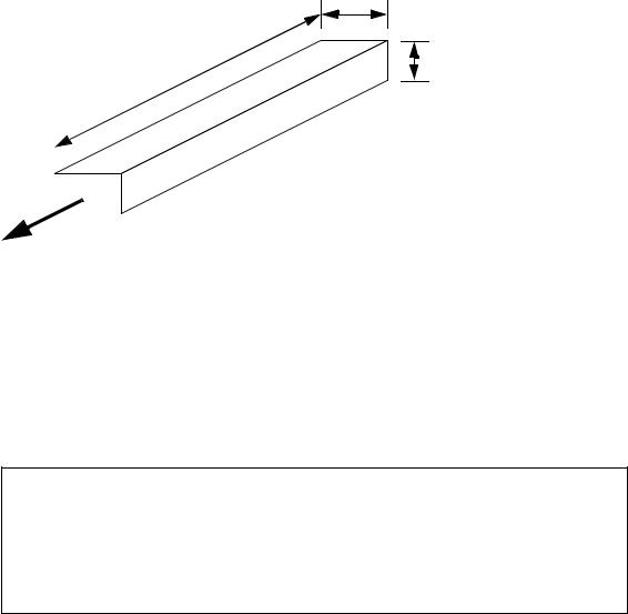
Strain gages measure strain in materials using the change in resistance of a wire. The wire is glued to the surface of a part, so that it undergoes the same strain as the part (at the mount point). Figure 14.16 shows the basic properties of the undeformed wire. Basically, the resistance of the wire is a function of the resistivity, length, and cross sectional area.
|
|
|
|
|
w |
|
|
|
|
|
|
|
|
|
|
|
|
|
|
|
|
|
|||
|
|
|
|
|
|
|
|
|
|
|
|
|
|
|
|
|
|
|
|
|
|
|
|
|
|
|
|
|
|
|
|
|
|
|
|
|
|
|
L |
|
|
|
|
- |
|
|
t |
|
|||
|
|
|
|
|
|
|
||||||
|
|
|
|
|
|
|
||||||
|
|
|
|
|
|
|
|
|
||||
|
|
|
|
|
|
|
|
|
||||
|
|
|
|
|
|
|
|
|
|
|||
|
V |
|
|
|
|
|
|
|
|
|
|
|
+ |
R = |
V |
|
L |
= ρ |
L |
||||||
-- |
= ρ -- |
----- |
||||||||||
|
|
|
I |
|
A |
|
|
|
wt |
|||
I
where, |
|
|
R |
= |
resistance of wire |
V, I |
= voltage and current |
|
L |
= |
length of wire |
w, t |
= width and thickness |
|
A |
= |
cross sectional area of conductor |
ρ |
= |
resistivity of material |
Figure 14.16 The Electrical Properties of a Wire
continuous sensors - 14.16
After the wire in Figure 14.16 has been deformed it will take on the new dimensions and resistance shown in Figure 14.17. If a force is applied as shown, the wire will become longer, as predicted by Young’s modulus. But, the cross sectional area will decrease, as predicted by Poison’s ratio. The new length and cross sectional area can then be used to find a new resistance.
w’
t’
L’
|
|
|
|
F |
|
F |
|
|
F |
|
|
|
|
|
σ |
= |
-- |
= |
----- |
= Eε |
ε = --------- |
|
|
|
|
|
|
|
|
A |
|
wt |
|
|
Ewt |
|
|
|
|
|
|
|
|
|
|
|
|
|
|||
|
|
|
|
L' |
|
|
|
L( 1 + ε) |
|
|
|
|
|
|
|
|
|
|
|
|
|
|
|||
|
|
|
|
------- |
|
---------------------------------------------- |
|
|
|
|||
|
|
R' = ρ w't' |
= ρ w( 1 – νε ) t( 1 – νε ) |
|
|
|
||||||
F |
|
|
|
|
|
|
( 1 + ε) |
|
|
|
||
|
|
∆ R = R' – R = R |
|
|
|
|
||||||
|
|
|
--------------------------------------- |
– 1 |
|
|||||||
|
|
|
( 1 – νε ) ( 1 – νε ) |
|
||||||||
|
|
where, |
|
|
|
|
|
|
|
|
||
|
|
|
|
ν |
= |
poissons ratio for the material |
||||||
|
|
|
|
F |
= applied force |
|
|
|
||||
|
|
|
|
E = Youngs modulus for the material |
||||||||
|
|
|
|
σ ,ε |
= |
stress and strain of material |
||||||
Aside: Gauge factor, as defined below, is a commonly used measure of stain gauge sensitivity.
∆ R
-------
R GF = ------------
ε
Figure 14.17 The Electrical and Mechanical Properties of the Deformed Wire
continuous sensors - 14.17
Aside: Changes in strain gauge resistance are typically small (large values would require strains that would cause the gauges to plastically deform). As a result, Wheatstone bridges are used to amplify the small change. In this circuit the variable resistor R2 would be tuned until Vo = 0V. Then the resistance of the strain gage can be calculated using the given equation.
V+ |
Rstrain |
= |
R2R1 |
when Vo = 0V |
|
------------- |
|
||
|
|
|
R3 |
|
R4
R2 |
|
|
|
|
R1 |
|
|
|
|||||
|
|
|
|
|
|
|
|
|
|
|
|
|
|
|
|
|
|
|
|
|
-
+
Vo
R3
Rstrain
R5
Figure 14.18 Measuring Strain with a Wheatstone Bridge
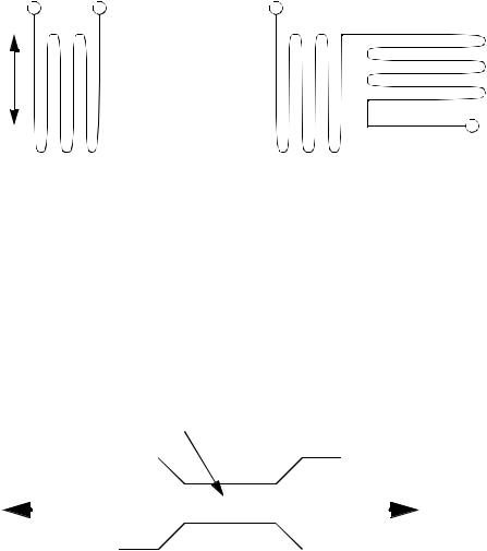
A strain gage must be small for accurate readings, so the wire is actually wound in a uniaxial or rosette pattern, as shown in Figure 14.19. When using uniaxial gages the direction is important, it must be placed in the direction of the normal stress. (Note: the gages cannot read shear stress.) Rosette gages are less sensitive to direction, and if a shear force is present the gage will measure the resulting normal force at 45 degrees. These gauges are sold on thin films that are glued to the surface of a part. The process of mounting strain gages involves surface cleaning. application of adhesives, and soldering leads to the strain gages.
continuous sensors - 14.18
stress |
irectiond |
uniaxial |
rosette |
Figure 14.19 Wire Arrangements in Strain Gages
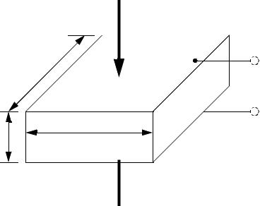
A design techniques using strain gages is to design a part with a narrowed neck to mount the strain gage on, as shown in Figure 14.20. In the narrow neck the strain is proportional to the load on the member, so it may be used to measure force. These parts are often called load cells.
mounted in narrow section to increase strain effect
F |
|
|
|
|
|
|
|
|
F |
|
|
|
|
|
|
|
|
|
|
|
|
|
|
|
|
|
|
|
|
|
|
|
|
|
|
|
|
|
|
|
|
|
|
|
|
|
|
|
|
|
|
|
|
|
Figure 14.20 Using a Narrow to Increase Strain
Strain gauges are inexpensive, and can be used to measure a wide range of stresses with accuracies under 1%. Gages require calibration before each use. This often involves making a reading with no load, or a known load applied. An example application includes using strain gages to measure die forces during stamping to estimate when maintenance is needed.
14.2.4.2 - Piezoelectric
When a crystal undergoes strain it displaces a small amount of charge. In other words, when the distance between atoms in the crystal lattice changes some electrons are forced out or drawn in. This also changes the capacitance of the crystal. This is known as
continuous sensors - 14.19
the Piezoelectric effect. Figure 14.21 shows the relationships for a crystal undergoing a linear deformation. The charge generated is a function of the force applied, the strain in the material, and a constant specific to the material. The change in capacitance is proportional to the change in the thickness.
F
b
+
q
-
|
εab |
d |
C = |
-------- |
---- |
c |
i = εgdtF |
where,
c |
a |
|
|
|
F |
C = capacitance change
a, b, c = geometry of material
ε = dielectric constant (quartz typ. 4.06*10**-11 F/m)
i = current generated
F = force applied
g = constant for material (quartz typ. 50*10**-3 Vm/N)
E = Youngs modulus (quartz typ. 8.6*10**10 N/m**2)
Figure 14.21 The Piezoelectric Effect
These crystals are used for force sensors, but they are also used for applications such as microphones and pressure sensors. Applying an electrical charge can induce strain, allowing them to be used as actuators, such as audio speakers.
When using piezoelectric sensors charge amplifiers are needed to convert the small amount of charge to a larger voltage. These sensors are best suited to dynamic measurements, when used for static measurements they tend to drift or slowly lose charge, and the signal value will change.