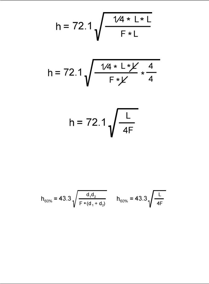
Step 3: Multiply the fractions in the numerator:

Step 4: Cancel the matching terms in the numerator and denominator and multiply by 4/4 to get the fraction out of the numerator:

Step 5: The result is the equation for the maximum first Fresnel zone radius (in feet) when the distance between transmitter and receiver (L) is given in statute miles and the frequency (F) is given in GHz.

The Erroneous Constant of Proportionality

Itʼs been shown, in excruciating detail, how the constant of proportionality for calculating the radius of the first Fresnel Zone is equal to 72.1. Weʼve also discussed that the first Fresnel zone must

be 60% unobstructed for proper signal reception. Sometimes youʼll see the Fresnel Zone formula presented with the constant of proportionality already adjusted to 60% of its proper value. This is a simple modification to the basic equation since 72.1 * .60 = 43.26, which is rounded up to 43.3, as shown in Figure 6.13, below.

Figure 6.13 The Typical Presentations of the Fresnel Zone Equations

Occasionally you will encounter an erroneous use of the constant of proportionality. A discussion of the radius of the first Fresnel zone will present the equations (using 43.3) for calculating the full size of the zone, and the accompanying literature will explain that this radius must be 60% unobstructed! Using the erroneous explanation results in calculating an unobstructed zone requirement that is 60% of 60% of the full first Fresnel zone radius, and not simply 60%. Itʼs hoped that the derivation of the Fresnel zone equations provided here will enlighten those who have erred in their understanding of the math. Itʼs probably the case that someoneʼs misunderstanding was taught to someone else who believed it to be factual. Then the misinformation spread as one writer, speaker, or technical instructor trusted that the equations they had learned were accurate. You now know the truth!

Copyright 2003 - Joseph Bardwell