

[Boyd]_cvxslides
.pdfLogistic regression
random variable y {0, 1} with distribution
exp(aT u + b) p = prob(y = 1) = 1 + exp(aT u + b)
• a, b are parameters; u Rn are (observable) explanatory variables
• estimation problem: estimate a, b from m observations (ui, yi)
log-likelihood function (for y1 = · · · = yk = 1, yk+1 = · · · = ym = 0):
l(a, b) = log |
|
1 + exp(aTiui + b) |
m |
1 + exp(aT ui + b) |
|
|
k |
|
|
|
|
|
Y |
exp(aT u + b) |
i Y |
1 |
|
|
|
|
|
||
|
i=1 |
|
=k+1 |
|
|
k |
|
m |
|
|
|
X |
|
X |
|
|
|
=(aT ui + b) − log(1 + exp(aT ui + b))
i=1 |
i=1 |
concave in a, b
Statistical estimation |
7–5 |

example (n = 1, m = 50 measurements) |
|
|
|||
|
1 |
|
|
|
|
|
0.8 |
|
|
|
|
= 1) |
0.6 |
|
|
|
|
(y |
|
|
|
|
|
prob |
0.4 |
|
|
|
|
|
|
|
|
|
|
|
0.2 |
|
|
|
|
|
0 |
|
|
|
|
|
0 |
2 |
4 u 6 |
8 |
10 |
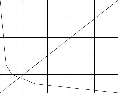
•circles show 50 points (ui, yi)
•solid curve is ML estimate of p = exp(au + b)/(1 + exp(au + b))
Statistical estimation |
7–6 |
(Binary) hypothesis testing
detection (hypothesis testing) problem
given observation of a random variable X {1, . . . , n}, choose between:
•hypothesis 1: X was generated by distribution p = (p1, . . . , pn)
•hypothesis 2: X was generated by distribution q = (q1, . . . , qn)
randomized detector
• a nonnegative matrix T R2×n, with 1T T = 1T
•if we observe X = k, we choose hypothesis 1 with probability t1k, hypothesis 2 with probability t2k
•if all elements of T are 0 or 1, it is called a deterministic detector
Statistical estimation |
7–7 |
detection probability matrix: |
|
|
|
|
|
|
Pfp |
1 − Pfn |
|||
D = T p T q = |
|
1 − Pfp |
Pfn |
|
|
•Pfp is probability of selecting hypothesis 2 if X is generated by distribution 1 (false positive)
•Pfn is probability of selecting hypothesis 1 if X is generated by distribution 2 (false negative)
multicriterion formulation of detector design
minimize (w.r.t. R+2 ) |
(Pfp, Pfn) = ((T p)2, (T q)1) |
subject to |
t1k + t2k = 1, k = 1, . . . , n |
|
tik ≥ 0, i = 1, 2, k = 1, . . . , n |
variable T R2×n |
|
Statistical estimation |
7–8 |
scalarization (with weight λ > 0)
minimize |
(T p)2 + λ(T q)1 |
subject to |
t1k + t2k = 1, tik ≥ 0, i = 1, 2, k = 1, . . . , n |
an LP with a simple analytical solution
(t1k, t2k) = |
(1, 0) |
pk ≥ λqk |
|
(0, 1) |
pk < λqk |
•a deterministic detector, given by a likelihood ratio test
•if pk = λqk for some k, any value 0 ≤ t1k ≤ 1, t1k = 1 − t2k is optimal (I.E., Pareto-optimal detectors include non-deterministic detectors)
minimax detector
minimize |
max{Pfp, Pfn} = max{(T p)2, (T q)1} |
subject to |
t1k + t2k = 1, tik ≥ 0, i = 1, 2, k = 1, . . . , n |
an LP; solution is usually not deterministic
Statistical estimation |
7–9 |
example |
|
0.20 |
0.10 |
|
P = |
||||
|
|
0.70 |
0.10 |
|
|
0.05 |
0.10 |
||
|
|
|
|
|
|
|
0.05 |
0.70 |
|
|
|
|
1 |
|
|
|
|
|
|
0.8 |
|
|
|
|
|
|
0.6 |
|
|
|
|
|
|
fn |
|
|
|
|
|
|
P |
|
|
|
|
|
|
0.4 |
|
|
|
|
|
|
0.2 |
1 |
|
|
|
|
|
2 |
4 |
|
|
|
|
|
|
3 |
|
|
|
||
0 |
|
|
|
|
|
|
|
0.2 |
0.4 Pfp |
|
0.8 |
1 |
|
0 |
|
0.6 |
solutions 1, 2, 3 (and endpoints) are deterministic; 4 is minimax detector
Statistical estimation |
7–10 |
Experiment design
m linear measurements yi = aTi x + wi, i = 1, . . . , m of unknown x Rn
• measurement errors wi are IID N (0, 1) |
|
|
||
• ML (least-squares) estimate is |
|
! |
|
|
xˆ = |
aiaiT |
−1 m |
yiai |
|
m |
|
|
|
|
X |
|
|
X |
|
i=1 |
|
|
i=1 |
|
• error e = xˆ − x has zero mean and covariance |
||||
E = E eeT = |
|
aiaiT |
! |
|
|
|
m |
−1 |
|
|
|
X |
|
|
|
|
i=1 |
|
|
confidence ellipsoids are given by {x | (x − xˆ)T E−1(x − xˆ) ≤ β}
experiment design: choose ai {v1, . . . , vp} (a set of possible test vectors) to make E ‘small’
Statistical estimation |
7–11 |
vector optimization formulation |
|
|
|
|
|
|
|
|
|
mk |
0, |
m1 + |
· · · |
|
|
p |
|
|
|
≥ P |
p |
|
|
−1 |
|
|
minimize (w.r.t. S+n ) E = |
k=1 mkvkvkT |
|
|
|
||||
subject to |
|
|
|
|
+ m = m |
|||
mk Z
•variables are mk (# vectors ai equal to vk)
•di cult in general, due to integer constraint
relaxed experiment design
assume m p, use λk = mk/m as (continuous) real variable
|
|
|
P |
|
|
|
−1 |
minimize (w.r.t. S+n ) |
E = (1/m) |
p |
|
λkvkvkT |
|||
|
=1 |
|
|||||
subject to |
λ 0, |
1T λ =k |
1 |
|
|
||
•common scalarizations: minimize log det E, tr E, λmax(E), . . .
•can add other convex constraints, E.G., bound experiment cost cT λ ≤ B
Statistical estimation |
7–12 |
D-optimal design |
|
P |
|
|
|
|
|
|
|
−1 |
|
minimize |
log det |
p |
λkvkvkT |
||
k=1 |
|
||||
subject to |
λ 0, |
1T λ = 1 |
|
||
interpretation: minimizes volume of confidence ellipsoids
dual problem
maximize |
log det W + n log n |
subject to |
vkT W vk ≤ 1, k = 1, . . . , p |
interpretation: {x | xT W x ≤ 1} is minimum volume ellipsoid centered at origin, that includes all test vectors vk
complementary slackness: for λ, W primal and dual optimal
λk(1 − vkT W vk) = 0, k = 1, . . . , p
optimal experiment uses vectors vk on boundary of ellipsoid defined by W
Statistical estimation |
7–13 |

example (p = 20)
λ1 = 0.5
λ2 = 0.5
design uses two vectors, on boundary of ellipse defined by optimal W
Statistical estimation |
7–14 |