[Boyd]_cvxslides

shape of penalty function has large e ect on distribution of residuals

Huber penalty function (with parameter M)

linear growth for large u makes approximation less sensitive to outliers

•left: Huber penalty for M = 1

•right: a ne function f(t) = α + βt fitted to 42 points ti, yi (circles) using quadratic (dashed) and Huber (solid) penalty

Least-norm problems

(A Rm×n with m ≤ n, k · k is a norm on Rn)

interpretations of solution x = argminAx=b kxk:

•geometric: x is point in a ne set {x | Ax = b} with minimum distance to 0

•estimation: b = Ax are (perfect) measurements of x; x is smallest (’most plausible’) estimate consistent with measurements

•design: x are design variables (inputs); b are required results (outputs) x is smallest (’most e cient’) design that satisfies requirements

examples

•least-squares solution of linear equations (k · k2): can be solved via optimality conditions

2x + AT ν = 0, Ax = b

• minimum sum of absolute values (k · k1): can be solved as an LP

φ : R → R is convex penalty function

Regularized approximation

minimize (w.r.t. R2+) (kAx − bk, kxk)

A Rm×n, norms on Rm and Rn can be di erent

interpretation: find good approximation Ax ≈ b with small x

•estimation: linear measurement model y = Ax + v, with prior knowledge that kxk is small

•optimal design: small x is cheaper or more e cient, or the linear model y = Ax is only valid for small x

•robust approximation: good approximation Ax ≈ b with small x is less sensitive to errors in A than good approximation with large x

Scalarized problem

minimize kAx − bk + γkxk

•solution for γ > 0 traces out optimal trade-o curve

•other common method: minimize kAx − bk2 + δkxk2 with δ > 0

Tikhonov regularization

minimize kAx − bk22 + δkxk22

can be solved as a least-squares problem

Optimal input design

linear dynamical system with impulse response h:

Xt

P

track desired output using a small and slowly varying input signal regularized least-squares formulation

minimize Jtrack + δJder + ηJmag

for fixed δ, η, a least-squares problem in u(0), . . . , u(N)

example: 3 solutions on optimal trade-o surface

(top) δ = 0, small η; (middle) δ = 0, larger η; (bottom) large δ

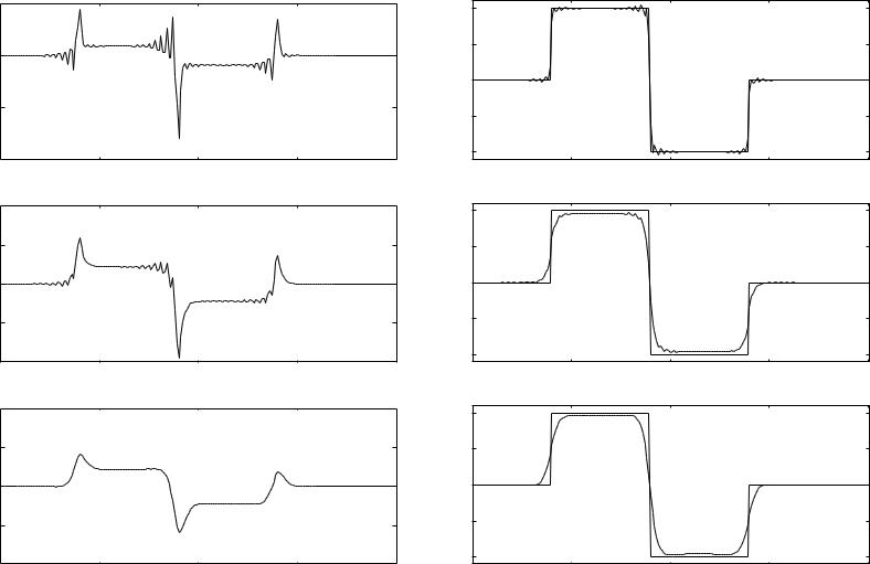
Signal reconstruction

minimize (w.r.t. R2+) (kxˆ − xcork2, φ(ˆx))

•x Rn is unknown signal

•xcor = x + v is (known) corrupted version of x, with additive noise v

•variable xˆ (reconstructed signal) is estimate of x

•φ : Rn → R is regularization function or smoothing objective

examples: quadratic smoothing, total variation smoothing:

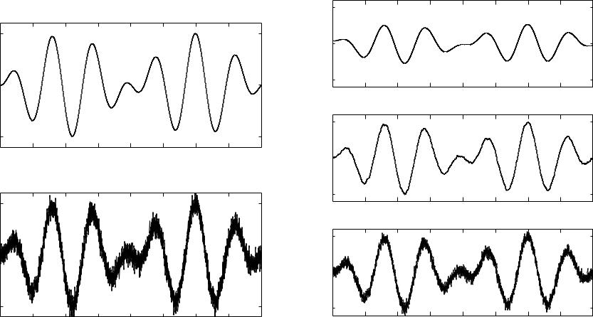
quadratic smoothing example