

28ANALYSIS AND VERIFICATION OF NON-REAL-TIME SYSTEMS
4.R(b)
5.A(y) M(y).
We can easily convert these clauses into clause set form, but here we start the proof by resolution from these clauses.
6.¬D(b, y)
7.¬O(a) D(b, a) resolvent of (3) and (4)
8.¬O(a) resolvent of (6) and (7)
9.¬A(a) resolvent of (1) and (8)
10.¬M(a) resolvent of (2) and (8)
11.M(a) resolvent of (5) and (9)
12. resolvent of (10) and (11)
Thus we have proved the validity of the original conclusion.
Chapter 6 applies some of these concepts to the analysis of safety assertions in relation to specifications expressed in real-time logic (RTL). RTL is a first-order logic that allows formulas to specify absolute occurrence time of events and actions.
2.2 AUTOMATA AND LANGUAGES
An automaton is able to determine whether a sequence of words belongs to a specific language. This language consists of a set of words over some finite alphabet. Depending on the type of automaton used, this sequence of words may be finite or infinite. If these sequences of words correspond to sequences of events and actions, we can construct an automaton that accepts correct sequences of events and actions in a system, and thus solve the verification problem as follows.
With the introduction of more concepts, we can use an automaton to represent a process or system. More precisely, a specification automaton represents the desired specification of a system, and an implementation automaton models an implementation attempting to satisfy the given specification. Our goal is to verify that the implementation satisfies the specification. This problem can now be viewed as the language inclusion problem (also known as the language containment problem), that is, to determine whether the language accepted by the implementation automaton is a subset of the language accepted by the specification automaton.
This section introduces several classical types of automata and the languages they accept. These automata are deterministic finite automata and nondeterministic finite automata. The languages include regular languages.
2.2.1 Languages and Their Representations
First, we define the terminology for languages. An alphabet is a finite set of symbols, which can be Roman letters, numbers, events, actions, or any object. A string
AUTOMATA AND LANGUAGES |
29 |
over an alphabet is a finite sequence of symbols selected from this alphabet. An empty string has no symbols and is denoted by e. The set of all strings over an alphabet is written as . The length of a string is the number of symbols in it. To refer to identical symbols at different positions in a string, we say these are occurrences of the symbol, just like saying instances (or iterations) of a process in a computer system.
The concatenation of two strings x1 and x2, written as x1x2, is the string x1 followed by the string x2. A subtstring of a string x is a subsequence of x. A language is any subset of . The complement, union, and intersection operations can be applied to languages since languages are sets. The language operation Kleene star (also called closure) of a language L, written as L , is the set of strings consisting of the concatenation of zero or more strings from L.
Now we describe how to use strings to represent languages. Since the set of strings over an alphabet is countably infinite, the number of possible representations of languages is countably infinite. However, the set of all possible languages over a given alphabet is uncountably infinite, and thus finite representations cannot be used to represent all languages. We next focus on languages that can be represented by finite representations. A regular expression specifies a language by a finite string consisting of single symbols, , possibly parentheses, and the symbolsand . We now define regular expressions more formally.
Regular Expressions: The regular expressions over an alphabet consist of the strings over the alphabet {), (, , , } such that:
1.Each member of and is a regular expression.
2.If α and β are regular expressions, then (α β) is a regular expression.
3.If α and β are regular expressions, then (αβ) is a regular expression.
4.If α is a regular expression, then α is a regular expression.
5.All regular expressions must satisfy the above rules.
Because every regular expression represents a language, we define a function L mapping from strings to languages such that for any regular expression α, L(α) is the language represented by α with the following properties.
1.For each a , L(a) = {a}, and L( ) = .
2.If α and β are regular expressions, then L((α β)) = L(α) L(β).
3.If α and β are regular expressions, then L((αβ)) = L(α)L(β).
4.If α is a regular expression, then L(α ) = L(a) .
2.2.2 Finite Automata
A deterministic finite automaton (DFA) belongs to a special class of finite automata in which their operation is completely determined by their input as described below. A DFA can be viewed as a simple language recognition device.
30 ANALYSIS AND VERIFICATION OF NON-REAL-TIME SYSTEMS
An input tape (divided into squares) contains a string of symbols, with one symbol in each tape square. The finite control is the main part of the machine whose internal status can be specified as one of a finite number of distinct states. Using a movable reading head, the finite control can sense the symbol written at any position on the input tape. This reading head is initially pointing to the leftmost square of the input tape and the finite control is set to the initial state. The automaton reads one symbol from the input tape at regular intervals and the reading head moves right to the next symbol on the input tape. Then the automaton enters a new state depending on the current state and the symbol read. These steps repeat until the reading head reaches the end of the input string. If the state reached after reading the entire string is one of the specified final states, the machine is said to accept the input string. The set of strings accepted by the machine is the language accepted by this machine. We now formally define a DFA.
Deterministic Finite Automaton: A deterministic finite automaton A is a 5-tuple
, S, S0, F, δ , in whichis a finite alphabet,
S is a finite set of states, S0 S is the initial state,
FS is the set of final states, and
δis the transition function from S × to S.
We can represent an automaton by a tabular representation called a transition table. For example, the transition table shown in Figure 2.9 represents an automaton that accepts strings in {a, b} with an odd number of bs. ρ is the current input symbol read. s is the current state of the automaton.
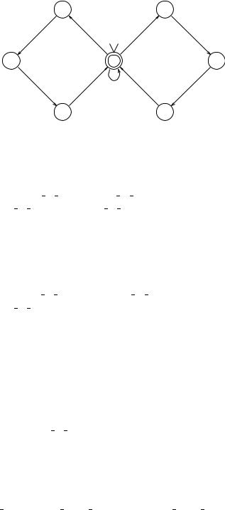
A clearer graphical representation of an automata is a state transition diagram (or simply state diagram), which is a labeled directed graph. In this graph, nodes represent states, and an edge (transition or arrow) is labeled with the symbol ρ from state s to state s if δ(s, ρ) = s . The initial state is indicated by a > or →. Final states, also called fixed points, are represented by double circles. The state transition diagram for the above automaton is shown in Figure 2.10. Figure 2.11 shows the transition table of an automaton that accepts strings in {a, b} with zero or an odd number of bs followed by zero or an even number of as. Figure 2.12 shows the corresponding automaton.
s |
ρ |
δ(s, ρ) |
|
|
|
s0 |
a |
s0 |
s0 |
b |
s1 |
s1 |
a |
s1 |
s1 |
b |
s0 |
Figure 2.9 Transition table 1.

AUTOMATA AND LANGUAGES |
31 |
|
a |
|
|
b |
|
a |
||
|
|
|
|
|
|
|
|
|
|
S0 |
|
|
b |
|
S1 |
||
|
|
|
|
|
|
|
|
|
|
Figure 2.10 |
Automaton A1. |
|
|||||
|
|
|
|
|
|
|
|
|
|
|
s |
ρ |
|
|
δ(s, ρ) |
|
|
|
|
|
|
|
|
|
|
|
|
|
s0 |
a |
|
|
s1 |
|
|
|
|
s0 |
b |
|
|
s3 |
|
|
|
|
s1 |
a |
|
|
s0 |
|
|
|
|
s1 |
b |
|
|
s2 |
|
|
|
|
s2 |
a |
|
|
s2 |
|
|
|
|
s2 |
b |
|
|
s2 |
|
|
|
|
s3 |
a |
|
|
s1 |
|
|
|
|
s3 |
b |
|
|
s4 |
|
|
|
|
s4 |
a |
|
|
s2 |
|
|
|
|
s4 |
b |
|
|
s3 |
|
|
|
Figure 2.11 Transition table 2. |
|||||||
S 0 |
a |
S 1 |
|
|
b |
S |
2 |
|
|
|
|
|
|
|
|
a,b |
|
|
|
|
|
|
|
|
|
|
|
a |
|
|
|
|
|
|
|
|
b |
a |
|
|
|
|
a |
|
|
|
|
|
b |
|
|
||
|
|
|
|
|
|
|
|
|
|
|
|
S 3 |
|
|
b |
S |
4 |
|
|
|
|
|
|
|
||
|
Figure 2.12 |
Automaton A2. |
|
|||||
To make finite automata more expressive, we introduce the feature of nondeterminism. A state change in a nondeterministic finite automaton (NFA) may be only partially determined by the current state and input symbol, and there may be more than one next state given a current state. Every nondeterministic finite automaton can be shown to be equivalent to a deterministic finite automaton, but this corresponding DFA usually contains more states and transitions. Hence, nondeterministic finite automata can often simplify the description of language recognizers.
32 ANALYSIS AND VERIFICATION OF NON-REAL-TIME SYSTEMS
Nondeterministic Finite Automaton: A nondeterministic finite automaton A is a 5-tuple , S, S0, F, , in which
is a finite alphabet,
S is a finite set of states, S0 S is the initial state,
F S is the set of final states, and
, the transition relation, is a finite subset of S × → S.
The class of languages accepted by finite automata is closed under concatenation, union, complementation, intersection, and Kleene star. We can prove each case by constructing a finite automaton α from one or two given finite automata. A language is regular iff it is accepted by a finite automaton. Let L(α), L(α1), and L(α2) be the languages accepted by automaton α, α1, and α2, respectively.
1.L(α) = L(α1) ◦ L(α2).
2.L(α) = L(α1) L(α2).
3.− L(α) is the complementary language accepted by deterministic finite automaton α , which is the same as α but with final and nonfinal states interchanged.
4.L(α1) ∩ L(α2) = − (( − L(α1)) ( − L(α2))).
5.L(α) = L(α1) .
Several important problems can be stated for finite automata, and the solutions to some of these problems can be derived using these closure properties. These problems are:
1.Given a finite automaton α:
(a)Is string t L(α)?
(b)Is L(α) = ?
(c)Is L(α) = ?
2.Given two finite automata α and β:
(a)Is L(α) L(β)?
(b)Is L(α) = L(β)?
The algorithms for solving the above problems are as follows. Suppose automaton α is deterministic. A nondeterministic finite automaton can always be transformed into a deterministic one.
Algorithm 1a executes automaton α on input t for a number of steps equal to the length of t. Because each step of α reads one input symbol, the state at which the automaton ends after length(t) steps determines whether t is accepted.
AUTOMATA AND LANGUAGES |
33 |
Algorithm 1b attempts to find, in the (finite) state transition diagram representing the automaton, a sequence of zero or more edges from the initial state to the final state. If there is no such path, then L(α) = .
Algorithm 1c checks with Algorithm 1b whether the language accepted by the complement of α is the empty set, that is, L(α ) = , where L(α ) = − L(α).
Algorithm 2a determines whether L(α) ∩ ( − L(β)) = using the property of closure under intersection and Algorithm 1b. If it is, then L(α) L(β).
Algorithm 2b employs Algorithm 2a twice to determine whether L(α) L(β) and
L(β) L(α).
Simulation is a powerful proof technique to show preorder, that an automaton, constructed from one or more automata of the same type, partially imitates the behavior of these other automata. For instance, we can simulate a nondeterministic finite automaton by a deterministic one. Bisimulation is another proof technique for checking equivalence, that the behaviors of two automata are identical. We describe automata-theoretic approaches for verifying the correctness of real-time systems in chapter 7.
2.2.3 Specification and Verification of Untimed Systems
We now show how an automaton can specify a physical system or a set of processes and how to determine whether a sequence of events or actions is allowed in the specified system. The alphabet of a language can consist of names of events or actions in the system to be specified. We call this alphabet the event set of the specified system. Then we can construct an automaton that accepts all allowable sequences (strings) of events in the specified system. This set of allowable sequences of events is the language accepted by this automaton. The following example illustrates these concepts by specifying a simplified automatic air conditioning and heating unit.
Example. The event set (the alphabet ) for the automatic climate-control (air conditioning and heating) automaton is {comfort, hot, cold, turn on ac, turn off ac, turn on heater, turn off heater}. The meanings of these events are as follows:
comfort: thermostat sensor detects the room temperature is within the comfort range, that is, between 68 and 78 degrees F.
hot: thermostat sensor detects the room temperature is above 78 degrees F. cold: thermostat sensor detects the room temperature is below 68 degrees F. turn on ac: turn on the air conditioner (cooler).
turn off ac: turn off the air conditioner (cooler). turn on heater: turn on the heater.
turn off heater: turn off the heater.
34 ANALYSIS AND VERIFICATION OF NON-REAL-TIME SYSTEMS
|
S4 |
|
|
|
S1 |
turn_on_heater |
|
|
cold |
|
hot |
|
|
|
|
|
|
S5 |
|
|
heater |
S0 |
|
|
|
|
|
turn |
|
|
|
_ |
|
||
|
|
|
_ |
||
|
|
off |
|
comfort |
|
|
|
|
_ |
||
|
_ |
|
|
off |
|
comfort |
|
|
|
||
turn |
|
|
|
ac |
|
|
|
|
|
||
|
S6 |
|
|
|
S3 |
turn_on_ac
S2
comfort
Figure 2.13 Automaton α for automatic air conditioning and heating system.
It is easy to show using Algorithm 1a whether a sequence of events is allowed in the specified system (Figure 2.13). For instance, the sequences
1a. comfort hot turn on ac comfort turn off ac and 1b. cold turn on heater comfort turn off heater
are accepted by the automaton α. Sequence (1a) states that when the sensor detects the temperature is too hot, the system activates the AC until a comfortable temperature is reached and then turns off the AC. Sequence (1b) states that when the sensor detects the temperature is too cold, the system activates the heater until a comfortable temperature is reached and then turns off the heater. However, the sequences
2a. comfort hot turn on heater comfort turn off heater and 2b. cold turn on heater comfort
are not accepted by the automaton α. Sequence (2a) states that when the sensor detects the temperature is too hot, the system activates the heater until a comfortable temperature is reached and then turns off the heater. Obviously, this should not be allowed since activating the heater makes the temperature even hotter. Sequence (2b) states that when the sensor detects the temperature is too cold, the system activates the heater until a comfortable temperature is reached but does not turn off the heater, which may make the temperature too hot.
Note that automata can only specify acceptable relative ordering of events in a sequence, but cannot specify absolute timing of events. In this example, we cannot specify that the event turn on ac must occur within, say, 5 seconds of the event hot. To handle absolute timing, we need to use timed automata, which will be introduced in chapter 7.
We next consider the specification and analysis of a more complex system: a smart traffic light system for a traffic intersection.
Example. This system has four components, each specified by an automaton: Pedestrian, Sensor Controller, Car Traffic Light, and Pedestrian Traffic Light.
AUTOMATA AND LANGUAGES |
35 |
When a pedestrian approaches the beginning of the pedestrian crosswalk for the traffic intersection, he/she is detected by a sensor controller. The sensor controller then sends a signal to the car traffic light to make it turn to red. This car traffic light turns to yellow and then to red, and in turn sends a signal to the pedestrian traffic light to make it turn on the “walk” sign. This walk sign should turn on before the pedestrian starts crossing the intersection.
Either the time interval for the walk sign to come on (after the pedestrian is detected by the sensor) is less than the time interval it takes to walk from the point the pedestrian is detected by the sensor to the start of the crosswalk, or the pedestrian waits for the walk sign to come on before starting to cross the intersection. Another sensor detects when the pedestrian finishes crossing and the sensor controller sends a signal to the pedestrian traffic light to make it turn to “don’t walk.” The pedestrian traffic light then turns to don’t walk and sends a signal to the car traffic light to make it turn to green.
The Pedestrian automaton communicates with the Sensor Controller automaton with the new pedestrian event to indicate a pedestrian approaches the intersec-
Pedestrian |
|
|
Sensor_Controller |
|
idle |
|
|
|
|
new_pedestrian |
S1 |
|
|
|
S0 |
|
|
|
|
|
|
|
no_pedestrian |
new_pedestrian |
no_pedestrian |
crossing |
S1 |
S0 |
S2 |
|
|
|
turn_don’t_walk |
turn_red |
S4 |
S2 |
|
idle |
|
|
|
|
||
end_crossing
|
Car_Traffic_Light |
Pedestrian_Traffic_Light |
|
|||
|
idle |
|
|
idle |
|
|
|
S0 |
turn_red |
S1 |
S0 |
is_red |
|
|
|
S1 |
|
|||
|
green |
|
yellow |
is_don’t_walk |
walk |
|
|
|
|
|
|
||
|
S5 |
|
S2 |
|
|
|
|
|
|
|
S4 |
S2 |
idle |
is_don’t_walk |
|
red |
|
|
|
|
|
|
|
|
don’t_walk |
turn_don’t_walk |
|
idle |
S4 |
is_red |
S3 |
|
S3 |
|
|
|
|
|
|
|
|
Figure 2.14 Smart traffic light system.

36 ANALYSIS AND VERIFICATION OF NON-REAL-TIME SYSTEMS
crossing, |
crossing, |
|
|
|
|
red |
(green V yellow) |
|
|
crossing, |
|
crossing, red |
(green V yellow) |
S2 |
S0 |
S1 |
|
green, crossing |
end_crossing, |
|
|
(green V yellow) |
|
Figure 2.15 Safety property for smart traffic light system.
tion. The events crossing and end crossing indicate the beginning and the end of the crossing by the pedestrian. The event of nothing happening is idle. The Sensor Controller automaton communicates with the Car Traffic Light automaton with the turn red event to signal it to turn red. Note that Car Traffic Light turns yellow before turning red. The Car Traffic Light automaton communicates with the Pedestrian Traffic Light automaton with the is red event to indicate that cars should have stopped and signal it to turn to walk.
When the pedestrian finishes crossing, the Pedestrian automaton communicates with the Sensor Controller automaton with the no pedestrian event to indicate a pedestrian leaves the intersection. The Sensor Controller automaton communicates with the Pedestrian Traffic Light automaton with the turn don’t walk event to signal it to turn to don’t walk. The Pedestrian Traffic Light automaton communicates with the Car Traffic Light automaton with the is don’t walk event to indicate that the pedestrian left the crosswalk and signal it to turn green. The entire system is shown in Figure 2.14. Figure 2.15 shows an automaton representing a desirable “safety property,” which is a requirement for the system to behave. Figure 2.16 shows the revised automaton for the Pedestrian to ensure that the system satisfies this safety property.
idle
new_pedestrian
S0 |
S1 |
no_pedestrian |
walk |
S3 |
S4 |
end_crossing |
crossing |
|
S2 |
Figure 2.16 Revised pedestrian automaton.