352 DESIGN AND ANALYSIS OF PROPOSITIONAL-LOGIC RULE-BASED SYSTEMS

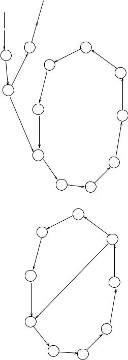
Figure 10.18 Traversing orders by the subrule 11.

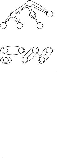
Figure 10.19 The ME graph of Program 3.

larly, N I12 = 1, N I21 = 5, N I22 = 1, N I31 = 7, N I32 = 2, N I41 = 1, N I51 = 1, N I61 = 1, and N I71 = 1.

Step 2 results in

N I1 = N I11 + N I12 = 7 + 1 = 8,

N I2 = N I21 + N I22 = 5 + 1 = 6,

N I3 = N I31 + N I32 = 7 + 1 = 8,

N I4 = N I41 = 1,

N I5 = N I51 = 1,

N I6 = N I61 = 1, and

N I7 = N I71 = 1.

The ME graph of Program 3 is then partitioned into four subgraphs by step 3, as shown in Figure 10.19. Finally, step 4 finds that

Tp = max(N I1, N I2) + max(N I3, N I5) + max(N I4) + max(N I6, N I7)

=8 + 8 + 1 + 1

=18.

10.12.11 The General Analysis Algorithm

In the previous sections, we showed the existence of two special forms and presented two algorithms to obtain upper bounds on the numbers of rule firings for programs in these two special forms. However, for any EQL program p, it is rarely the case that p as a whole is in a known special form. Instead, it is frequently found that p can

Proof of Theorem 6. Assume p is in Special Form D and does not always reach a fixed point in a bounded number of rule firings. This means that an execution of p exists that does not terminate in any bounded number of rule firings. Since only a finite number of rules in p exist, a rule r1 must be firing infinitely often during this execution. According to the underlying execution model, r1 can be fired only if its firing changes the value of one variable in p. Since only a finite number of variables in Lr 1 exist, a variable x1 Lr 1 must be assigned a new value by a subrule ri1 infinitely often.

Based on the values of Rp ∩ L p and Tp ∩ L p , we divide the proof into four parts. To simplify the notations used next, the notation ri is used to stand for the specific subrule of the rule ri that assigns a value to a variable involved in the reasoning, unless otherwise stated. For example, without ambiguity, the subrule ri1 will be referred to as r1.

1.Rp ∩L p = and Tp ∩L p = . p is also a Special Form A program. According to Theorem 5, p always reaches a fixed point in a bounded number of rule firings.

2.Rp ∩ L p = and Tp ∩ L p = . Due to Rp ∩ L p = , r1 always assigns the constant value m1 to x1. r1 alone can change the value of x1 at most once if

another subrule does not exist that assigns a different value to x1. Hence, there must be a rule r1 with a subrule r1 that assigns a distinct value m1 to x1 and is fired infinitely often.

Due to (D1), r1 and r1 mutually exclude each other. There must be a vari-

the pair of r2 and r2 . We continue to apply the same arguments to the variables

and rules encountered.

Two paths, S = rk , rk−1, . . . , r2, r1 and S = rk , r(k−1)

will be found. However, since there are only a finite number of rules (and thus subrules) in p, eventually, for some k, both rk and rk will turn out to be subrules already encountered previously. One of three situations will happen:

(a)rk {rk−1, rk−2, . . . , r2, r1} and rk {r(k−1) , r(k−2) , . . . , r2 , r1 }.

Assume rk = ri and rk = r j . Then rk = ri , rk−1, . . . , ri+1, ri

(k−1) , . . . , r( j+1) , r j forms another

are respec-

tively contained in disjoint simple cycles and assign distinct values to xk , contradicting (D4).

(b)Both rk and rk belong to {rk−1, rk−2, . . . , r2, r1}. There are two cases to consider:

assigned to x remains disabled throughout this execution of p. The fact that r1 assigns a new value to x infinitely often means that f changes its value infinitely often. Hence, f must be a function in at least one variable such that it can change its value, otherwise it is a constant expression and cannot change its value. Only two possible situations exist for f to be a function in variables. We now discuss both situations and prove they cannot occur.

(b) f is a function in a variable y that is different from the variable x (i.e., r is of the form x := f (y) | · · · IF EC). There is a subrule r1 of the form x := f (y) IF EC, and y (and thus f (y)) changes its value infinitely often. There must be a rule r2 (and a subrule r2) assigning a value to y and firing infinitely often. Now, the argument applied to r1 also applies to r2. We continue to apply the same argument to each rule encountered. Eventually, since there are only a finite number of rules in p, the subrules encountered form a cycle C in GRDp . Since the subrules in C can be fired one after another infinitely often, C is not a convergency cycle and all of the subrules in C are enabled at the same time, violating (D5). Hence, this situation cannot occur either.

Since neither of the two situations can possibly happen, it is not possible for p not to reach a fixed point in a bounded number of rule firings if Rp ∩ L p =

if (1) the value of f1 has changed such that it is not equal to the old value of x1 or (2) a new value has been assigned to x1 by another rule, say r1 , such that the new value of x1 is not equal to the value of f1. There are two cases involving the value of f1: constant or not constant.

• f1 is a constant expression. This means r1 can change the value of x1 at most once if another rule does not exist assigning a distinct value to x1. Since r1 assigns a new value to x1 infinitely often, there must be another rule r1 assigning a distinct value to x1 infinitely often. r1 and r1 mutually exclude each other, due to (D1). Hence, a variable x2 exists whose value changes infinitely often and determines the enabledness of r1 and r1 . That, in turn, means there is a rule r2 that assigns a new value to x2 infinitely often and potentially enables r1. Hence, the ER edge r2, r1 exists in GRDp . Now, the argument applied to the pair of x1 and r1 also applies to the pair of x2 and r2.

• f1 is not a constant expression. f1 must be a variable expression either in x1 or not x1.

358 DESIGN AND ANALYSIS OF PROPOSITIONAL-LOGIC RULE-BASED SYSTEMS

thus f (x2)) changes infinitely often. A rule r2 may exist that

assigns a new value to x2 and fires infinitely often. Hence, there is a VM edge r2, r1 in GRDp . Now, the argument ap-

plied to the pair of r1 and x1 also applies to the pair of r2 and x2.

We continue to apply the argument above to each rule and variable pair encountered. A path of ER edges or VM edges or both will be found. Eventually, since only a finite number of rules exist in p, a rule and variable pair that has been encountered previously will be encountered again. Hence, a cycle C will be found. One of three situations will happen (to simplify the explanation, if a variable x is assigned a value by a subrule in C, we say x is in C):

(a)C is an EV cycle. However, the existence of an EV cycle would violate (D2). Thus, this situation will not occur.

(b)C is an ER cycle. For each pair of ri and xi in C, the value of fi assigned to xi by ri is a constant. This means that xi is also assigned

a distinct value infinitely often by another rule ri that enables r(i−1) . Hence, the ER edge ri , r(i−1) also exists in GRDp . A path consisting

of ri , r(i−1) , . . . , r2 , r1 in GRDp shall also exist. Since there are only a finite number of rules in p, eventually we will end up with the same

situation as we did in part (2) of this proof. That means this situation will not occur either.

(c)C is a VM cycle. For each variable xi in C, xi gets a new value because the expression f (xi+1) assigned to xi by ri changes infinitely often. Since the subrules in C can be fired one after another in the order they

appear in C for an unlimited number of times, it is obvious that C is

not a convergent cycle. In addition, for each subrule ri in C, ri must be enabled at the time when it is ri ’s turn to be fired. If all of the subrules in C can be enabled at the same time, then (D5) is violated. On the other hand, if all of the subrules (vertices) contained in C cannot be

enabled at the same time, there must be at least one disabled rule at any

moment. Assume rk is disabled at some moment during the execution considered. Hence, there must be a subrule, say g1, whose firing will enable rk . There are two cases to consider: