

12 Physics of imaging
Contents
Treatment of contrast media reaction 839
Iodinated contrast 840
Gadolinium-based contrast 842
Physics quick review 844
e
nucleus
outer shell
e
 e
e
1)outer shell electron is ejected
2)photon is scattered with:
longer wavelength lower frequency lower energy
838
Treatment of contrast media reaction
non-allergic-type acute contrast reactions
-type |
Hypotension and bradycardia (vasovagal) |
|
1. ECG, pulse oximetry, blood pressure |
||
-allergic |
||
2. Oxygen via facemask |
||
rg |
||
non |
||
|
||
moderate |
5. If poorly responsive, atropine 0.6−1 mg IV |
|
May repeat up to 0.04 mg/kg (2.8 mg for 70 kg) |
||
6. Call for assistance (at any point) |
||
mild to |
|
-type |
Bronchospasm |
|
2. Oxygen via facemask |
||
allergic |
||
|
1. ECG, pulse oximetry, blood pressure |
|
- |
3. Beta-agonist inhalers |
|
non |
||
4. If poorly responsive: |
||
severe |
||
Epinephrine IM 1:1,000, 0.1−0.3 ml (0.1−0.3 mg) |
||
|
||
to |
or |
|
Epinephrine IV 1:10,000, 1−3 ml (0.1−0.3 mg) |
||
moderate |
||
May repeat up to 1 mg |
||
|
||
|
5. Call for assistance (at any point) |
-type |
Pulmonary edema |
|
2. Oxygen via facemask |
||
allergic |
||
|
1. ECG, pulse oximetry, blood pressure |
|
- |
3. Elevate torso |
|
non |
4. Furosemide 20−40 mg IV |
|
severetomoderate |
||
5. Call for assistance (at any point) |
||
|
-type |
Seizures |
|
2. Oxygen via facemask |
||
allergic |
||
|
1. ECG, pulse oximetry, blood pressure |
|
- |
3. Consider diazepam 5 mg IV |
|
non |
or |
|
severe |
||
midazolam 0.5−1 mg IV |
||
|
||
to |
4. Continue to monitor vitals and pulse oximetry |
|
5. Call for assistance (at any point) |
||
moderate |
||
|
allergic-type acute contrast reactions
Urticaria (hives)
type- |
1. Discontinue injection if not completed |
|
|
||
allergic |
2. If mild, no treatment |
|
3. If moderate, diphenhydramine PO/IV 25−50 mg |
||
|
||
moderatetomild |
4. If severe: |
|
Epinephrine IM 1:1,000, 0.1−0.3 ml (0.1−0.3 mg) |
||
|
||
|
5. Call for assistance (at any point) |
-type |
Facial or laryngeal edema |
|
1. ECG, pulse oximetry, blood pressure |
||
allergic |
||
3. Epinephrine IM 1:1,000, 0.1−0.3 ml (0.1−0.3 mg) |
||
|
2. Oxygen via facemask |
|
severeto |
or |
|
May repeat up to 1 mg |
||
|
Epinephrine IV 1:10,000, 1−3 ml (0.1−0.3 mg) |
|
moderate |
4. Call for assistance (at any point) |
|
|
Hypotension and tachycardia (anaphylaxis)
1.ECG, pulse oximetry, blood pressure
2.Oxygen via facemask
-type |
|
Trendelenburg |
|
5. |
If poorly responsive: |
||
allergic |
|||
|
Epinephrine IV 1:10,000, 1 ml (0.1 mg) |
||
|
|
||
severe |
|
May repeat up to 1 mg |
|
6. |
Call for assistance (at any point) |
||
|
839

Iodinated contrast
Iodinated contrast media reaction
Contrast media reaction overview
•Acute reactions to intravenous contrast can be divided into allergic-type and non- allergic-type mechanisms. Both allergic-type and non-allergic-type reactions can range in severity from mild and self-limited to severe and life-threatening.
•Patients with asthma are at increased risk of an allergic reaction to contrast medium.
•A seafood or shellfish allergy is not associated with allergic reaction to contrast.
•Mild nausea, sensation of warmth, and flushing are considered physiologic and are not adverse reactions to contrast.
Mild contrast reactions
•A mild contrast reaction is self-limited and does not require medical management.
•A vasovagal reaction to intravenous contrast is rare and is characterized by bradycardia and hypotension. Mild vasovagal reactions are usually self-limited and are not allergic in etiology.
•Urticarial reactions are mild allergic-type reactions, and include hives and mild angioedema. The symptoms of mild angioedema include scratchy throat, slight tongue or facial swelling, and sneezing, and generally do not require medical management.
Moderate contrast reactions
•Moderate contrast reactions are not immediately life-threatening but may require medical management.
•Moderate allergic-type reactions include severe urticaria, bronchospasm, moderate tongue/facial swelling, and transient hypotension with tachycardia.
•Moderate non-allergic-type reactions include significant vasovagal reaction, pulmonary edema, bronchospasm, and limited seizure.
Severe contrast reactions
•Severereactionstointravenousiodinatedcontrastmaybeimmediatelylife-threatening.
•Allergic-type severe reactions include anaphylaxis and angioedema. Symptoms may be varied and include altered mental status, respiratory distress, diffuse erythema, severe hypotension, or cardiac arrest.
•Non-allergic-type severe reactions include severe pulmonary edema, severe bronchospasm, and severe seizure.
Premedication to prevent contrast reaction
•In a patient with a known contrast allergy, a repeat contrast reaction is most likely to be similar to the prior reaction. However, the repeat reaction may be either more or less severe. Therefore, if IV contrast is necessary for a patient who has had a previous reaction, a premedication regimen is recommended, although contrast reactions may occur despite premedication. Intravenous contrast is generally contraindicated in patients who have had a prior severe allergic-type reaction.
•Elective premedication: Prednisone 50 mg PO at 13 hours, 7 hours, and 1 hour before the exam, plus diphenhydramine 50 mg (IV or PO) 1 hour before.
•Emergentpremedication:Hydrocortisone200mgIVQ4h,1–2timespriortoadministration ofIVcontrast.Diphenhydramineisgiven1hourprior.NotethatIVsteroidshavenot been
showntobeeffectivewhengivensoonerthan4hoursbeforethecontrastadministration.
840

Contrast-induced nephropathy (CIN)
Risk of contrast-induced nephropathy (CIN)
•Contrast-inducednephropathy(CIN)isadecreaseinrenalfunctionofunknownetiology followingtheintravascular(venousorarterial)administrationofiodinatedcontrast.
•The most important risk factor for development of CIN is preexisting renal insufficiency.
•For patients with eGFR <30 ml/min/1.73m2, the risk of CIN is between 7.8 and 12.1%.
•For patients with eGFR >30 and <45, the risk of CIN is between 2.9 and 9.8%.
•For patients with eGFR >45 and <60, the risk of CIN is between 0 and 2.5%.
•The development of CIN in patients with normal renal function (eGFR >60 ml/ min/1.73m2) is exceptionally rare.
•Note that gadolinium-based contrast media are not known to cause contrast-induced nephropathy.
•Patients with multiple myeloma are at increased risk of irreversible renal failure after receiving high-osmolality contrast media from tubular protein precipitation. There are no data on the risk of the low or iso-osmolar contrast agents in current use.
Prevention of contrast nephropathy
•The main preventative strategies against CIN are to use the minimal dose of contrast possible and to adequately hydrate the patient. The use of sodium bicarbonate and N-acetylcysteine has been previously advocated but the effectiveness of these agents has not been proven.
•Patients with an eGFR >30 and <60 typically receive approximately 2/3 the standard contrast dose. Administration of intravenous contrast to a patient with an eGFR <30 would require a careful assessment of risks and benefits on a case by case basis.
•The standard dose of intravenous iodinated contrast can generally be given to patients on dialysis. Careful attention should be paid to the volume status in these patients as theoretically the osmotic load increases intravascular volume.
Iodinated CT contrast: General considerations
Iodinated contrast and pheochromocytoma
•It is safe to administer nonionic contrast media to patients with pheochromocytoma. Prior studies showed an increased in serum catecholamines after high-osmolality contrast agents, which are no longer in current use.
Iodinated contrast and thyroid uptake
•Thyroid gland uptake of I-131 is reduced to about 50% one week after iodinated contrast injection. Therefore, if radioactive I-131 therapy is planned, iodinated contrast should be avoided for a few weeks prior to I-131 therapy.
Metformin and intravenous contrast
•Metforminisanoralanti-hyperglycemicagentthatdecreaseshepaticglucoseproduction andincreasesperipheralglucoseuptake.Althoughexceptionallyrare,thereisanincreased riskofmetformin-associatedlacticacidosisinpatientsreceivingintravenousiodinated contrast,thoughttobeduetoCINandtheresultantaccumulationofmetformin.
•There is no need to discontinue metformin in patients with normal renal function. In patients with multiple comorbidities, metformin should be discontinued at time of contrast administration and withheld for 48 hours.
•Note that it is not necessary to discontinue metformin prior to gadolinium-based contrast.
841

Iodinated contrast and pregnancy
•Iodinated contrast crosses the placenta and enters the fetal circulation. No mutagenic or teratogenic effects have been observed; however, no controlled studies in pregnant patients have been performed.
•It is acceptable to administer iodinated contrast to a pregnant patient if medically necessary. It is recommended that a pregnant patient sign an informed consent form prior to undergoing an examination involving ionizing radiation and iodinated contrast.
Iodinated contrast and breast feeding
•The plasma half-life of iodinated contrast is approximately 2 hours. Less than 1% of the administered maternal dose of iodinated contrast is excreted in the breast milk within 24 hours of maternal administration, and 1% of that dose may be absorbed by the infant’s gastrointestinal tract. The total infant absorbed dose is therefore approximately 0.01% of the administered maternal dose.
•Breast feeding mothers do not need to halt breast feeding. If the mother is concerned, abstaining from breast feeding for 24 hours (while pumping and discarding milk) would result in effectively zero fetal dose.
Contrast extravasation
•Extravasation is the leakage of contrast into the soft tissues at the injection site. Although the risk of extravasation is not related to the injection flow rate, the use of automatic injectors can lead to a large extravasated volume of contrast media.
•Iodinated contrast is toxic to the soft tissues and skin, although serious adverse events are relatively rare following extravasation. The most common serious injury due to contrast extravasation is compartment syndrome. Less commonly, skin ulceration and tissue necrosis can occur.
•All patients with extravasation should be evaluated by the radiologist. Elevation of the extremity to decrease capillary hydrostatic pressure has been recommended, but is without supporting data. There is no evidence favoring warm or cold compresses, and both are used commonly.
•Surgical consultation should be obtained for progressive swelling and pain, altered tissue perfusion (decreased capillary refill), change in sensation, or skin ulceration or blistering.
Gadolinium-based contrast
Immediate adverse reactions to gadolinium-based contrast
•Both mild and severe adverse reactions to gadolinium-based contrast are much more rare compared to iodinated contrast. Most adverse reactions to gadolinium-based contrast are mild such as nausea, vomiting, headache, or pain at the injection site.
•Allergic-type reactions to gadolinium are rare, seen in 0.004% to 0.7%
•Serious anaphylactic reactions are exceeding rare (<0.01%).
Contrast extravasation
•Gadolinium-based contrast agents are much less toxic to the skin and soft tissues compared to iodinated contrast.
•Evaluation and treatment of extravasation is similar for both types of contrast.
842

Nephrogenic systemic fibrosis (NSF)
•Nephrogenic systemic fibrosis (NSF) is a highly morbid disease characterized by diffuse fibrosis of the skin and subcutaneous tissues, which may also involve the visceral organs.
•NSF is strongly associated with gadolinium exposure in patients with reduced renal function. The exact mechanism for development of NSF is unknown, but may involve dissociation of toxic free gadolinium in patients with reduced renal clearance. The free gadolinium may bind phosphate and precipitate in tissues, inducing a fibrotic reaction.
•Patients with end-stage renal disease (eGFR <30 ml/min/1.73m2) have between 1% and 7% chance of developing NSF even after a single exposure to a gadoliniumcontaining contrast agent. There has been only one established case of NSF developing in a patient with an eGFR >30.
•In general, gadolinium-based contrast should not be given to patients on renal dialysis or with eGFR <30. Although it is exceedingly rare for NSF to develop in a patient with eGFR between 30 and 59, eGFR may fluctuate daily in these patients. For this reason, caution should be employed for patients on the lower end of this spectrum.
•Different brands and formulations of gadolinium-based contrast are associated with varying rates of NSF.
Gadolinium-based contrast in pregnancy and breast-feeding
Gadolinium-based contrast and pregnancy
•Gadolinium-based contrast should not be administered during pregnancy. Gadolinium-based contrast crosses the placenta. Although never demonstrated to cause harm, gadolinium chelates may accumulate in the amniotic fluid and remain there indefinitely, with risk of dissociation of toxic free gadolinium ion.
Gadolinium-based contrast and breast feeding
•The plasma half-life of gadolinium-based contrast is 2 hours. Less than 0.04% of the administered maternal dose is excreted in the breast milk within 24 hours of maternal administration, and 1% of that dose may be absorbed by the infant’s gastrointestinal tract. The total infant absorbed dose of gadolinium is therefore approximately 0.0004% of the administered maternal dose.
•It is likely safe for the mother to continue breast feeding. There is no information to suggest that oral ingestion of such a tiny amount of gadolinium-containing contrast may be harmful to the fetus.
Contrast media reference:
ACR Committee on Drugs and Contrast Media (2012). ACR Manual on Contrast Media Version 8. Retrieved from http://www. acr.org/Quality-Safety/Resources/Contrast-Manual, accessed September 2012.
843
Physics quick review
Measuring radiation
Exposure, air kerma, absorbed dose, equivalent dose, and effective dose
•Exposure is the charge of electrons liberated per unit mass of air. Exposure is measured in Coulombs/kg.
•Air kerma (kinetic energy released per mass) describes the incident X-ray beam intensity as the kinetic energy transferred from uncharged particles (photons) to charged particles (electrons). Air kerma is measured in Gray (J/kg).
•Air Kerma (Gy) can be converted to absorbed dose (also quantified in Gy) by the R factor, which depends on kV and the atomic number (Z) of the absorbing tissue.
Bone (Z = 12) absorbs much more energy than soft tissue (Z ~ 7.6).
At 10 mGy air kerma, bone absorbs 40 Gy, tissue absorbs 11 Gy.
•The equivalent dose (expressed in Sievert; Sv) is the absorbed dose in Gy multiplied by a radiation weighting factor (WR).
WR depends on the linear energy transfer (LET) of the type of radiation. For diagnostic radiology using X-rays, WR = 1. An alpha particle has a high LET.
•The effective dose (also expressed in Sv) is an estimation of radiation exposure that takes into account the equivalent dose to all organs exposed and each organ’s radiosensitivity.
Effective dose = the sum of the absorbed dose (Gy) * WR * WT for all organs exposed.
WT is the tissue weighting factor, which varies from 0.12 for radiosensitive organs (e.g., bone marrow, colon, lung, breast), to 0.01 for less sensitive organs (e.g., bone, brain, and skin).
Radiation |
• SI (Système International) units including Gray and Sievert are almost universally |
|
units |
used rather than the older non-SI units. One notable exception is the Curie, which is |
|
|
still commonly used in nuclear medicine (typical dosing ranges are in millicuries). |
|
|
SI (Système international) units |
Non-SI units |
|
• Gray (Gy) quantifies both absorbed |
• 1 Rad (radiation absorbed dose) = 10 mGy |
|
dose and air kerma (exposure) as |
|
|
energy absorbed per unit mass. |
|
|
• 1 Gy = 1 J/kg |
|
|
• 1 Gy = 100 Rad |
|
|
• Sievert (Sv) is used to quantify |
• 1 Rem = 10 mSv |
|
equivalent dose and effective dose. |
|
|
• 1 Sv = 100 Rem |
|
|
• A Becquerel (Bq) is only used in |
• 1 Curie = 37 billion Becquerels = |
|
nuclear medicine for radioactive |
3.7e10 disintegrations per second |
|
materials. |
|
• 1 Bq = 1 disintegration per second
844
General radiography
X-ray generator |
• X-ray photons are generated when high-energy electrons hit a target at the |
|
anode side of the circuit. For general radiography and CT, the target is made of |
|
tungsten (atomic symbol W). |
|
99% of the electrons’ kinetic energy is converted to heat, and 1% is converted to X-rays. |
|
• 90% of X-rays are produced from bremsstrahlung (nuclear field interaction). |
|
The maximum keV (energy) of the X-ray spectrum is the kV of the generator. The average |
|
keV ~ 1/3 max. |
|
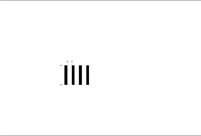
• 10% of X-rays are produced from characteristic radiation. A characteristic X-ray |
|
is produced when a high energy electron knocks a K-shell electron out of orbit. |
high-energy electron comes in high-energy photon comes out
energetic electron needs to have keV > K-shell binding energy
e
K shell
e
nucleus
e
outer shell
e |
2) outer shell electron fills vacancy |
|
3) characteristic X-ray produced |
||
|
||
1) K-shell |
E = E(K-shell) −E(transition shell) |
|
|
||
electron |
|
|
ejected |
|
characteristic x-rays are produced with energies just below K-shell binding energy.
No characteristic X-rays are generated when kV < K-edge
•Tungsten: Atomic weight = 74; K-edge = 70 keV; characteristic X-rays <70 keV.
Effect of kV on tube output • X-ray production is proportional to (kV)2.
•In practice, changing kV is complicated as a change in kV causes a change in characteristic X-ray, shifts spectrum to the right, and adds photons.
•h kV by 15% g h photons by 100%.
•In general, increasing kV will decrease dose and decrease contrast when automatic exposure control is used.
Heel effect |
• The heel effect is due to attenuation • |
The main contributor to the |
|
at the anode, causing fewer X-rays |
heel effect is the anode angle |
|
at the anode side. |
(typical anode angle ~15 |
|
|
degrees). |
|
|
i anode angle g h heel effect |
845
X-ray interactions with matter
All of these interactions deal with incoming photons.
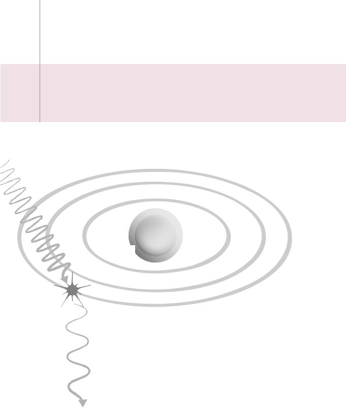
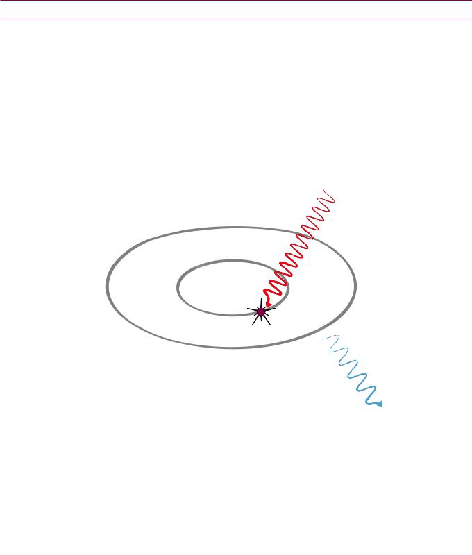
•Coherent scatter: No exchange of energy, no change in frequency, and no contribution to patient dose. Contributes less than 5% of X-ray interactions.
E = energy of incoming |
|
photon (keV) |
• Compton scatter: Proportional to (electron density)/E. Scattered photons |
|
go in all directions. |
|
Compton scatter dominates at >25 keV in soft tissue and >40 keV in bone. |
e
nucleus
outer shell
e
|
e |
|
|
1) outer shell electron is ejected |
|
|
2) photon is scattered with: |
|
|
longer wavelength |
|
|
lower frequency |
|
Z = electron number |
lower energy |
|
• Photoelectric effect: Proportional to Z3/E3. |
||
|
Photoelectric effect dominates at <25 keV in soft tissue and <40 keV in bone.
outer shell
(intermediate shells not shown)
K shell
e
nucleus
2) inner shell electron ejected
e
1) incident photon absorbed
e
4) characteristic X-ray or Auger electron produced (not diagrammed)
Energy from the ejected inner shell electron is absorbed locally (energetic electrons don’t travel very far); however, a 30 keV electron can cause significant damage via 1,000 ionizations (approximately 30 eV/ionization).
846
Linear attenuation coefficient
µ (cm–1)
•N = N0 *e–µt
fraction transmitted = e–µt
•If µ is “small” (<0.1/cm), then µ
is the proportion of photons that interact with matter.
•If µ is “large” (>0.1/cm), then the formula above is used.
N0 = initial number of photons
N = transmitted number of photons after thickness t
This is only true for weakly attenuating material.
Example: If µ = 0.5/cm, then e–µt = 61% transmitted.
Mass attenuation |
• |
Mass attenuation coefficient = (µ/ρ), where ρ = density |
coefficient |
• Because density is accounted for in the formula above, the mass attenuation |
|
|
||
|
|
coefficient is independent of density. |
|
|
|
Scatter and grids |
• |
In radiography, the typical scatter:primary ratio is 5-10:1 |
|
• |
Scatter i contrast |
• Grid ratio = height/width
Typical grid ratios in radiography are between 8 and 12 (the height of the grid is 8–12 times the width between grid elements).
W
H
• About 70% of primary radiation passes through the grid.
• Bucky factor is the relative h dose due to grid = incident/transmitted
radiation
The Bucky factor should not be confused with the grid ratio!
Typical Bucky factor is 5–10 (e.g., h mAs from 40 g 200).
•h kV will h scatter (Compton effects dominate at higher kV).
•Grids not used for extremity radiography (bone is h Z and not very thick).
Beam quality and half value layer (HVL)
•A “high quality” beam has low-energy photons filtered out.
•The half-value layer (HVL) is a measurement of the beam quality and is the thickness of material that attenuates 50% of the incident energy.
•HVL is dependent on photon energy. HVL h with h photon energy.
•Aluminum (Al) is the standard material for measuring HVL.
•Typical HVL for mammography is 0.3 mm Al.
•Typical HVL for radiography is 3 mm Al.
State regulations require beam quality: HVL >2.5 mm Al at 80 kVp.
•Typical HVL for CT is 8–9 mm Al.
847
Film optical density (OD)
and characteristic curves
•Film optical density (OD) = log10(I0/It) = log10(incident/transmitted light intensity)
OD of 1 g 10% photons transmitted through film
OD of 2 g 1% transmitted
OD of 3 g 0.1% transmitted
•Film “looks good” if the average OD is ~ 1.5. This occurs after approximately 5 µGy photons hit the film/screen.
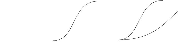
•A characteristic curve logarithmically plots the relationship between radiation exposure (air kerma) and film optical density.
The toe is the low-exposure region and the shoulder is the high exposure region. Fog is the baseline low-level darkening of film that occurs in the absence of radiation exposure.
•Latitude is the range of air kerma with satisfactory film density. A highlatitude film is ideal for imaging body parts with a wide variation of X-ray transmission (e.g., a chest radiograph). A high-contrast (low-latitude) film is ideal for accentuating image contrast in tissues with low subject contrast (e.g., mammography).
• Gamma is steepest part of curve; |
• Effect of latitude on characteristic |
||||||||||||
gradient is average steepness: |
|
curve: |
|
|
|||||||||
|
3 |
|
|
|
|
shoulder |
|
3 |
|
|
high-contrast |
||
|
|
|
|
|
|
|
|
|
|
|
|
||
density |
|
|
|
|
region |
density |
|
|
|
(mammo) |
|||
2 |
|
|
|
2 |
|
|
high-latitude |
||||||
|
|
|
|
|
|||||||||
|
|
|
|
|
|
|
|
|
|
(CXR) |
|||
optical |
|
|
|
linear |
|
|
|
optical |
1 |
|
|
|
|
1 |
|
|
|
|
|
|
|
|
|
|
|||
|
|
toe |
|
base + fog ~ 0.2 OD |
|
|
|
|
|
||||
|
|
|
|
|
|
|
|
||||||
|
|
|
|
|
|
|
|
|
|
||||
|
|
|
|
|
|
|
|
|
|
|
|
|
|
|
|
|
|
|
|
|
|
|
|
|
|
log(exposure) |
|
|
|
|
|
log(exposure) |
|
|
|
|
|||||
Digital detectors
All except Xe are Solid State detectors.
CsI and Selenium used without cassette.
•Ionization chamber: High-pressure Xe (k-edge 35 keV): Used for measuring radiation, not for imaging.
•Photostimulable phosphor: Barium fluorohalide (BaFBr); used in computed radiography.
Read out with red laser light (emits blue light).
Dynamic range is 10,000:1 (vs. 40:1 for screen-film).
Can be used with air kerma <0.1 µGy to 1,000 µGy.
•Scintillator: Cesium Iodide (CsI); note that CsI also used as input phosphor in an
image intensifier.
Indirect: Absorbed X-rays first converted to light, which is then stored as charge. Advantage: K-edge 30-ish, good at absorbing X-rays.
Disadvantage: Light spreads out g blur
•Photoconductor: (Selenium)
Direct: Absorbed X-rays directly converted to charge.
Advantage: No light spreading, very sharp.
Disadvantage: K-edge 13, poor X-ray absorber at standard radiography keV.
Used in digital mammography.
848

Mammography physics
Contact mammography |
• |
kV is reduced to h contrast |
• 25 kV; 100 mA (HVL 0.3 mm Al) |
|
technique summary |
• |
Focal spot is smaller |
• 0.3 mm focal spot standard |
|
|
||||
|
|
|
100 mA tube current |
|
|
|
|
• 0.1 mm magnification focal spot |
|
|
|
|
25 mA tube current |
|
|
• |
h h photons deposited on detector, |
• 200 µGy (vs. 5 µGy for standard |
|
|
|
resulting in lower noise |
radiography) |
|
|
• |
h exposure |
• 1 s vs. 50 ms for abdominal X-ray |
|
|
• |
h mAs |
• 100 mAs vs. ~20 mAs (abdominal |
|
|
|
|
radiograph) |
|
|
• |
Grid ratio smaller |
• 5:1 (PE > Compton, less scatter) |
|
|
|
|
Bucky factor ~2 |
|
|
• |
Film gradient h |
• 3 vs. 2 |
|
|
• |
Higher luminance viewboxes |
• 3,000 cd/m2 is ACR requirement |
|
|
• Single-emulsion films used |
|
||
|
• |
Heel effect taken advantage of |
• Cathode side directed to chest wall |
|
Compared to |
• |
Contrast increased by: i kV, breast compression, h gamma film |
||
traditional |
• Resolution improved by: Single thin screen, small focal spot, compression |
|||
radiography, |
||||
• |
Noise (mottle) reduced by: h photons at image receptor (200 µGy vs. 5 µGy |
|||
mammography image |
||||
quality improved by |
|
for screen-film) |
|
|
several factors |
|
|
|
|
|
|
|
||
Mammography X-ray |
• |
Molybdenum (Mo) target (K-edge 20 keV) generates characteristic X-rays at |
||
generator and filters |
|
17 and 19 keV. |
|
|
•Mo filter i i low-energy X-rays (which do not contribute to imaging but add to radiation exposure) and i high frequency X-rays (which i contrast).
Mo filter lets characteristic X-rays through.
•Average energy generated ~ 17 keV (typical rule that average energy ~1/3 to 1/2 max doesn’t apply since characteristic X-rays are so much more important).
•Rhodium (Rh) filter shifts spectrum to the right, used for thicker/denser breasts.
•Rh target/Rh filter used in conjunction for even thicker breasts.
Breast compression |
• Advantages of breast compression: |
|
h X-ray penetration |
|
h density uniformity |
|
i scatter |
|
i dose |
|
i tissue overlap |
|
i focal spot blur |
•Disadvantages of compression:
May be uncomfortable
849
Digital mammography |
• Pixel size ~80 µm; smallest visible microcalcifications ~ 150 µm |
|||||||||||
|
• Resolution ~ 3,000 × 4,000 pixels = 24 MB at 2 byte/pixel |
|||||||||||
|
• 5 megapixel monitors needed for viewing |
|||||||||||
|
|
|
|
|
|
|
|
|
|
|
|
|
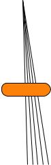
Magnification |
• Magnification = SID/SOD |
|||||||||||
Mammography |
SID = source–image distance |
|||||||||||
|
||||||||||||
|
SOD = source–receptor distance |
|||||||||||
|
• SID typically 65 cm, SOD typically 35 cm |
|||||||||||
|
In the example below, SID = 65 cm, SOD = 35 cm, and magnification = 65/35 = 1.85 |
|||||||||||
|
|
|
|
|
|
|
|
|
|
|
||
|
65 cm |
SOD = 35 cm |
|
|
|
|||||||
|
SID = |
|
|
|
|
|
|
|
|
|||
|
30 cm |
|
|
|
|
|
||||||
|
|
|
|
|||||||||
|
|
|
OID = |
|
|
|||||||
|
|
|
|
|
|
|
|
|
|
|
||
|
|
|
|
|
|
|
|
|
|
|
|
|
|
|
|
|
|
|
|
|
|
|
|
|
|
|
OID = Object–image distance |
|||||||||||
|
• If h SID (X-ray tube moved away) then exposure time will be too long. |
|||||||||||
|
• If i SID (X-ray tube moved closer) then there will be too much focal spot |
|||||||||||
|
blur. |
|
|
|
|
|
|
|
|
|
|
|
|
• No grid needed (air gap introduced). |
|||||||||||
|
• 0.1 mm focal spot used. |
|||||||||||
|
• Magnification mammography technique summary: |
|||||||||||
|
25 mA current |
|||||||||||
|
3 second exposure |
|||||||||||
|
70 mAs. Because a grid is not employed, a lower total mAs is needed (compared to 100 |
|||||||||||
|
mAs with contact mammography using a grid. |
|||||||||||
|
|
|||||||||||
MQSA |
• The interpreting physician needs to have read 960 mammograms in the |
|||||||||||
|
prior 24 months. |
|||||||||||
|
• A quality control program must be in place. |
|||||||||||
|
• Phantom must be tested weekly with an average glandular dose <3 mGy. |
|||||||||||
|
|
|||||||||||
Average glandular dose |
• Federal requirement that AGD <3 mGy per view per breast. |
|||||||||||
(AGD) |
Note that the fluoroscopic dose limit of 100 or 200 mGy/minute is the only other |
|||||||||||
|
federal dose regulation. |
|||||||||||
• A typical AGD is ~ 1.8–1.5 mGy per view per breast (digital slightly lower
dose).
850

Fluoroscopy physics
Electronic |
• If field of view (FOV) is i by a factor of two (e.g., from 10 cm to 5 cm), the |
||
magnification |
reduced field of view is projected onto the entire output phosphor of the |
||
|
image intensifier, which will be 4 times dimmer. Therefore, skin exposure will |
||
|
be increased by a factor of 4 by the automatic exposure control. |
||
|
• Similarly, reducing the exposed area from 10 cm to 7 cm would increase |
||
|
patient entrance air kerma by a factor of two. |
||
|
|
|
|
Fluoro technique |
• Continuous fluoro runs at current of 1 to 5 mA (typically 3 mA), resulting |
||
|
in a very low air kerma/frame of approximately ~0.01 µGy. Compared to a |
||
|
standard chest X-ray exposure of 5 µGy, each fluoro frame has 500 times |
||
|
fewer incident photons. |
||
|
• There is a federal regulatory limit of 100 mGy/min entrance air kerma. |
||
|
High-dose fluoro with audible/visual alarms allows 200 mGy/min for large patients. |
||
|
|
|
|
Effects of fluoroscopy |
• Increasing source to skin distance decreases dose due to inverse-square law. |
||
techniques on dose |
• Increasing filtration reduces dose by removing low-energy X-rays that would |
||
|
|||
|
be absorbed. |
||
|
• Removing grid reduces dose (used in peds), at the risk of increasing scatter. |
||
|
• Dose spreading (moving the beam around) reduces the maximum skin dose. |
||
|
Skin dose rate is about 10–30 mGy/min for continuous fluoroscopy. |
||
|
Maximum exposure rate 100 mGy/min or 200 mGy/min in high-level mode. |
||
|
At maximum permissible rate in high-level mode, 2 Gy can be delivered in 10 min! |
||
|
Large patients are more susceptible to skin injury. |
||
|
• Magnification increases dose, as discussed above. |
||
|
|
|
|
CT physics |
|
|
|
Overview of CT |
• Computed tomography (CT) produces images by rotating a fan beam around |
||
|
the patient and determining the linear attenuation coefficients of each |
||
|
individual pixel using a reconstruction algorithm. |
||
|
|
|
|
Hounsfield units (HU) |
• A Hounsfield unit is a measure of relative CT attenuation. |
||
|
HU = 1,000 ( |
µx – µwater |
) |
|
µwater |
||
|
µx = attenuation coefficient of the material being measuring |
||
|
µwater = attenuation coefficient of water |
||
|
• 10 HU = 1% difference in contrast. |
||
|
• Gray matter and white matter differ in contrast by only 0.5%. |
||
|
• A material with twice the attenuation of water attenuates 1,000 HU. |
||
851

Radiation dosimetry
CT dosimetry |
• |
The computed tomography dose index (CTDI) is the average phantom dose |
|
|
for a single axial slice (one complete rotation without table motion), including |
|
|
scatter, measured in Gy. |
|
|
CTDI is measured with 16 cm and 32 cm phantoms. 16 cm will always have higher dose. |
|
• CTDIw (weighted) = 2/3 CTDIp + 1/3 CTDIc |
|
|
|
CTDIp = peripheral |
|
|
CTDIc = central |
|
• |
CTDIvol = CTDIw/pitch |
The pitch is related to the table speed. A pitch <1 will overscan and result in increased radiation exposure; conversely, a pitch >1 will skip areas but will decrease exposure.
CTDIvol is the same for all scans, independent of scan length. CTDIvol should be less than reference values:
Adult head: 75 mGy (16 cm phantom)
Adult abdomen: 25 mGy (32 cm phantom)
Pediatric abdomen: 20 mGy (16 cm phantom)
Dose length product (DLP) and effective doses
•The dose length product (DLP) is the best way to estimate radiation risk from CT.
•DLP = CTDIvol * scan length = mGy*cm
•One can obtain an effective dose in mSv from the DLP by using body-part specific conversion factors:
Head 0.0023 mSv/mGy cm
Neck 0.0054
Chest 0.019
Abd 0.017
Pelvis 0.017
Legs 0.0008
•Example conversion: If DLP is 900 mGy*cm for an abdominal CT, the radiation exposure equals (900 mGy*cm) * (0.017 mSv/mGy cm) = 15.4 mSv.
Typical effective |
• |
Radiography: |
• |
Interventional radiology: |
doses (mSv) of |
|
PA and lateral chest radiograph: 0.1 mSv |
|
Cerebral angiography: 1–10 mSv |
common diagnostic |
|
|
||
|
Cervical spine radiograph: 0.2 mSv |
|
Peripheral angiography: 5 mSv |
|
exams |
|
|
||
|
Lumbar spine radiograph: 1.5 mSv |
|
Cardiac cath (diagnostic): 7 mSv |
|
|
|
|
||
|
|
Abdomen radiograph: 0.7 mSv |
|
TIPS: 100 mSv |
|
|
Pelvic radiograph: 0.6 mSv |
• |
CT: |
|
|
Mammography: 0.4 mSv |
|
Head CT: 2 mSv |
|
• |
Knee radiograph: 0.005 mSv |
|
Neck CT: 3 mSv |
|
Fluoroscopy: |
|
Chest CT: 7 mSv |
|
|
|
Upper GI series: 6 mSv |
|
Abdomen CT: 8 mSv |
|
|
Barium enema: 8 mSv |
|
Pelvis: 6 mSv |
852

Image quality
Contrast |
• The most important factor for optimizing contrast is to increase the number of |
|||
|
|
photons that reach the film (film density). |
|
|
|
• i scatter g h contrast |
|
|
|
|
• Collimation i scatter and i dose |
|
|
|
|
|
Collimation is the rare example of something that h image quality and i dose |
||
|
• h kV g i contrast with automatic exposure control |
|
||
|
• In screen film, contrast is related to screen latitude/gradient. |
|||
|
|
|||
Resolution and blur |
• Only three factors influence blur (resolution), none of which affects image |
|||
|
|
contrast: |
|
|
|
|
1) Focal spot blur. |
|
|
|
|
2) Motion blur, which is related to exposure time. |
|
|
|
|
3) Receptor blur, which is related to intensifying screen thickness. Faster screens h blur. |
||
|
|
|
|
|
Statistics |
|
|
|
|
Sensitivity, |
• |
Sensitivity = TP/(TP + FN) |
• |
TP = true positive |
specificity, positive |
• |
Specificity = TN/(TN + FP) |
• |
TN = true negative |
predictive value, |
• |
Positive predictive value (PPV) = TP/(TP + FP) |
• |
FP = false positive |
and negative |
||||
predictive value |
• |
Negative predictive value (NPV) = TN/(TN + FN) |
• |
FN = false negative |
|
|
|||
ROC curve |
• A receiver operator characteristic (ROC) curve compares the diagnostic |
|||
|
|
performance of a test at various thresholds of decision confidence. |
||
decision threshold
# patients
“negative” |
“positive” |
normals abnormals
TN TP
FN FP
thresh2 thresh1
parameter for decision threshold
true positive fraction 100%
0
ROC curve
thresh2
thresh1
100%
false positive fraction
•A patient population includes normals and abnormals. The threshold to determine whether a test parameter is “negative” or “positive” can be set to optimize the ratio of true positives to false positives.
•In threshold 1 (thresh1; blue dashed line above), the decision threshold is chosen to balance true positives with false positives. This threshold is visualized on the ROC curve as the blue dot.
•Threshold 2 (thresh2; brown dashed line above) is lowered. When plotted on the ROC curve, thresh2 moves to the right, which increases the true positive fraction (increases sensitivity) and also increases the false positive fraction.
853
Radiation biology
DNA damage |
• Free radicals mediate the majority of biological damage due to radiation. |
||
|
|
|
|
Syndromes |
• Xeroderma pigmentosa: |
• |
Ataxia telangiectasia: |
|
h sensitivity to UV light |
|
h sensitivity to X-rays |
|
|
||
Deterministic effects |
• Deterministic effects occur once the radiation exposure crosses a certain |
||
|
threshold and would not be expected to occur below that exposure. |
||
|
• A decrease in peripheral lymphocyte count can occur after as little as ≥0.5 |
||
|
Gy exposure. |
|
|
|
• Cataracts may occur after an eye dose of 2 Gy. The posterior pole is |
||
|
preferentially affected. For a given dose, high-LET radiation (neutrons and |
||
|
alpha particles) are much more effective at inducing cataracts compared to |
||
|
X-rays. |
|
|
|
• Radiation-induced erythema can occur in 1–2 days, but may take up to |
||
|
10–14 days to develop. |
|
|
|
2 Gy: Transient early erythema |
|
|
|
6 Gy: Robust erythema |
|
|
|
• Epilation occurs after about 3 weeks. |
|
|
|
3 Gy: Temporary epilation |
|
|
|
7 Gy: Permanent epilation |
|
|
|
• Desquamation may begin 4 weeks after exposure. |
||
|
15 Gy: Moist desquamation |
|
|
|
• Vascular damage is expected for skin doses >20 Gy. |
||
|
• Ulceration and depigmentation are late effects due to dermal damage. |
||
|
• Sterility can be caused in males or females. |
|
|
|
Males: Temporary sterility after >0.15 Gy. |
|
|
|
Females: Permanent sterility and early menopause after >3.5 Gy. |
||
|
|
||
Hereditary effects |
• The doubling dose is the dose required to double the spontaneous mutation |
||
|
rate when applied to a population. The doubling dose is approximately 1 Gy |
||
|
given to each member of the population. |
|
|
• The risk of hereditary effects (for an individual) is thought to be approximately 0.2% per Sv. For instance, the risk of a hereditary effect from a gonad dose of 100 mSv = 0.2% * 0.1 Sv = 0.02%.
Death by radiation
(whole-bodyradiation)
Terminology: LD 50/X = lethal dose that kills 50% of the population in X days. For instance, an LD 50/60 will kill 50% of the population in 60 days.
•3–4 Gy: LD 50/60 due to failure of hematopoietic system.
•10 Gy: LD 50/5 due to denuding of the GI tract lining (small bowel most sensitive).
•100 Gy: LD 50/2 due to cerebrovascular syndrome.
854

Stochastic effects |
• Stochastic effects are random and carcinogenic. Stochastic effects arise after |
|
a latent period of several years. As the dose to an individual increases, there |
|
is an increased risk of developing cancer. Complicating the determination of a |
|
stochastic risk is the fact that cancer is a very common disease, there is a low |
|
level of background radiation present, and most people who receive medical |
|
radiation exposures do not have any ill effects. |
|
• The risk of a stochastic effect depends on the dose, dose rate, and type of |
|
tissue exposed. |
|
• The linear no threshold model is believed to provide the most accurate risk |
|
assessment for development of solid tumors, with a latency up to 25 years. |
|
The linear no threshold model assumes that there is no threshold required |
|
for a stochastic effect, and the risk of cancer increases linearly with increasing |
|
exposure. |
|
• The linear-quadratic function of dose is thought to best characterize the risk |
|
of developing leukemia, with a latency of 5–7 years. |
Radiation-induced cancer
•Acute radiation exposure carries a risk of developing cancer of approximately 8%/Gy, based on Japanese nuclear bomb survivors.
For instance, a 24% increase in cancer risk would require 4 Gy acutely (8 *4 = 24%).
•The risk of leukemia is approximately 1%/Sv for an acute dose.
•Chronic exposure (e.g., radiation worker) carries a risk of cancer of 4%/Gy.
Relative |
• The thyroid gland is the most radiosensitive tissue in the human body. |
radiosensitivities |
|
Occupational/ iatrogenic exposures and effects
•Ankylosing spondylitis (treated with X-rays) g leukemia
•Fluoroscopy for tuberculosis g breast cancer
•Marshall island inhabitants (nuclear weapon testing) g thyroid tumors
•Miners (especially uranium) g lung cancer, due to breathing radon
•Dial painters g bone sarcomas and nasopharyngeal carcinoma (lick radium on brushes)
Radiation effects on the fetus
These effects are for significant exposure (e.g., 2 Gy)
•Weeks 0–2 (pre-implantation): “all-or-nothing”: abortion likely after significant exposure
•Weeks 2–6: congenital abnormalities
h Risk of neonatal death (death at or about the time of birth)
•Weeks 8–15: Risk of mental retardation 40%/Sv h Risk of childhood cancer
h Risk of reduced head diameter
•Weeks 15–25: Risk of mental retardation 10%/Sv h Risk of childhood cancer
Fetal dose |
• |
Dose limit: 0.5 mSv/month allowed (~5 mSv/pregnancy). |
|
(Pregnant radiation |
• |
Lead apron attenuates externally measured dose by a factor of 20 (fetal dose |
|
workers) |
|||
|
would be further reduced by factor of 2 due to mother’s overlying tissues). |
||
|
|
855

Dose to general public |
• 1 mSv/year, which is actually lower than the maximum dose of 5 mSv |
|
allowed by medical |
allowed to the fetus of a radiation worker. |
|
radiation |
|
|
|
|
|
Dose limits by body part |
• Eyes: 150 mSv/year |
• Everything else: 500 mSv/year |
|
|
|
Occupational exposure |
• Max permissible effective dose = 50 mSv/year |
|
(not pregnant) |
|
|
|
|
|
Background radiation |
• Background radiation varies by location, but averages about 3 mSv/year |
|
|
excluding medical radiation. |
|
1 Gy (Sv) is required to double the mutation rate, so 3 mSv = 0.003 Sv = 0.3% increased risk of mutation above the baseline rate.
•Radon exposure represents approximately 55% of background radiation. Radon is an alpha emitter with a half-life of 3 days. Its parent radionuclide is radium, with a half life of 1,600 years.
Effective dose = Absorbed dose * WR * WT
WR = 20 (h LET), and WT = 0.1 (only lung tissue irradiated)
Radon exposure is thought to cause ~20,000 deaths/year.
Magnetic resonance imaging (MRI) physics
MRI and |
• Although no controlled studies have been performed, MRI can be performed at |
|
pregnancy |
any stage of pregnancy. Gadolinium is contraindicated throughout pregnancy. |
|
|
|
|
MRI quenching |
• Quenching causes loss of superconductivity of the MRI scanner magnet coils, |
|
|
which releases helium. Helium displaces O2 g must evacuate emergently. |
|
|
|
|
Fringe field |
• The fringe field surrounds the controlled access area and cannot exceed 5 Gauss. |
|
|
|
|
FDA regulates the |
• Static magnetic field strength >4T. |
|
following MRI |
• Time-varying magnetic fields sufficient to produce severe discomfort or painful |
|
parameters |
||
stimulation. |
||
|
||
|
• Radiofrequency power deposition to produce core temperature increase of 1 |
|
|
degree C. |
|
|
• Acoustic noise levels >140 dB. |
SAR
Specific absorption ratio
•The specific absorption ration (SAR) characterizes the radiofrequency (RF) power absorbed per unit mass.
•SAR is proportional to number of images acquired per unit time and depends on patient dimensions, RF waveform, tip angle, and coil type.
MRI noise |
• The acoustic noise produced by the MRI scanner is caused by vibrating gradient |
|
coils, due to rapidly applied gradient magnetic fields. |
856

Focal heating and thermal injuries
•Conductive loops can cause local heating. Examples of conductive loops include crossed arms, ECG leads, and unconnected surface coil leads in contact with patient’s skin.
•Metallic objects can absorb radiofrequency energy and become hot.
•Time-varying magnetic fields can result in peripheral nerve stimulation, muscle movement, and discomfort.
Signal to noise |
• Signal to noise ratio (SNR) is proportional to: I * voxelx,y,z * |
NEX |
* B |
|
ratio (SNR) |
||||
BW |
||||
|
|
|
||
|
I = intrinsic signal intensity of voxel, dependent on tissue composition and pulse sequence |
|||
|
voxelx,y,z = voxel volume, affected by image matrix and slice thickness |
|
|
|
|
A smaller voxel volume will proportionally decrease signal to noise |
|
|
|
|
NEX = number of excitations; linearly related to time of acquisition |
|
|
|
|
BW = receiver bandwidth (range of frequencies collected by the MRI system; wide BW enables |
|||
|
faster data acquisition and reduces chemical shift artifacts but also adds noise g reduces SNR) |
|||
|
B = intrinsic function of magnetic field strength |
|
|
|
|
|
|||
T1 and T2 |
• Inherent tissue T1 and T2 characteristics depend on the longitudinal relaxation |
|||
(T1) and transverse relaxation (T2) times of the protons in that tissue.
• Tissue signal abnormality is produced by alterations (prolongation or shortening) of the transverse or longitudinal relaxation of the tissue, which may be affected by various pathologic processes.
• MR image weighting (e.g., T1or T2-weighted images) depends on the repetition time (TR) and echo time (TE) used to obtain images.
• T1 image contrast is dependent on TR, which is the interval between sequential radiofrequency pulses. The imaging appearance of specific tissues on T1-weighted images depends on how much longitudinal relaxation occurs between each TR.
Images obtained with a short TR and a short TE are T1-weighted.
Short T1 relaxation times g higher signal on T1-weighted images.
Fat and subacute blood have short T1 relaxation times and therefore appear hyperintense on T1-weighted images.
• T2 image contrast is dependent on TE, which is the interval between the application of the radiofrequency pulse and the collection of the signal. The imaging appearance of tissues on T2-weighted images depends on how much transverse relaxation (loss of proton phase coherence) occurs during each TE. Images obtained with a long TR and a long TE are T2-weighted.
Slow loss of phase coherence g prolonged T2 relaxation times g hyperintense on T2weighted images.
Water has a long T2 relaxation time and therefore is hyperintense on T2-weighted images.
857

T1
Short TR
Short TE
T2
Long TR
Long TE
PD
Long TR
Short TE
Highest SNR i contrast
relative signal intensity
relative signal intensity
relative signal intensity
|
|
|
|
|
longitudinal relaxation (T1) |
|
|
|
|
|
|
|
|
|
|
|
|
|
transverse relaxation (T2) |
|
|
||||||||||||||||||||||||||
1.0 |
|
|
|
|
|
|
|
|
|
|
|
|
|
|
|
|
|
|
|
|
|
|
1.0 |
|
|
|
|
|
|
|
|
|
|
|
|
|
|
|
|
|
|
|
|
|
|
|
|
|
|
|
|
|
|
|
|
fat |
|
|
|
|
|
|
|
|
|
|
|
|
|
|
|
|
|
|
|
|
|
|
|
|
|
|
|
|
|
|
|
|
|
|
|
|
|||
0.8 |
|
|
|
|
|
|
|
|
|
|
|
|
|
|
|
|
|
|
|
|
0.8 |
|
|
|
|
|
|
|
fat |
|
|
|
|
|
|
|
|
|
|||||||||
|
|
|
|
|
|
|
|
|
|
|
|
|
|
|
|
|
|
|
|
|
|
|
|
|
|
|
|
|
|
|
|
|
|
|
|
||||||||||||
|
|
|
|
|
|
|
|
|
|
|
|
|
|
|
|
|
|
|
|
|
|
|
|
|
|
|
|
|
|
|
|
|
|
|
|
|
|
||||||||||
|
|
|
|
|
|
|
|
|
|
|
|
|
|
|
|
|
|
|
|
|
|
|
|
|
|
|
|
|
|
|
|
|
|
|
|
||||||||||||
0.6 |
|
|
|
|
|
|
|
|
|
|
|
|
|
|
|
|
|
|
|
|
|
|
0.6 |
|
|
|
|
|
|
|
|
|
|
|
|
|
|
|
|
||||||||
|
|
|
|
|
|
|
|
|
|
|
|
|
|
|
|
|
|
|
|
|
|
|
|
|
|
|
|
|
|
|
|
|
|
|
|
|
|
||||||||||
|
|
|
|
|
|
|
|
|
|
|
|
|
|
|
|
|
|
|
|
|
|
|
|
|
|
|
|
|
|
|
|
|
|
||||||||||||||
|
|
|
|
|
|
|
|
|
|
|
|
|
|
|
|
|
|
|
|
|
|
|
|
|
|
|
|
|
|
|
|
|
|
|
|
|
|
|
|
|
|
|
|
|
|
||
|
|
|
|
|
|
|
|
|
|
|
|
|
|
|
|
|
|
|
|
|
|
|
|
|
|
|
|
|
|
|
|
|
|
|
|
|
|
|
|
|
|
|
|
||||
0.4 |
|
|
|
|
|
|
|
water |
|
|
|
|
|
|
|
|
|
|
|
|
0.4 |
|
|
|
|
|
|
|
|
|
water |
|
|
|
|
|
|
|
|
|
|||||||
|
|
|
|
|
|
|
|
|
|
|
|
|
|
|
|
|
|
|
|
|
|
|
|
|
|
|
|
|
|
|
|
|
|
|
|
|
|||||||||||
|
|
|
|
|
|
|
|
|
|
|
|
|
|
|
|
|
|
|
|
|
|
|
|
|
|
|
|
|
|
|
|
|
|
|
|||||||||||||
0.2 |
|
|
|
|
|
|
|
|
|
|
|
|
|
|
|
|
|
|
|
0.2 |
|
|
|
|
|
|
|
|
|
|
|
|
|
|
|
|
|
|
|||||||||
|
|
|
|
|
|
|
|
|
|
|
|
|
|
|
|
|
|
|
|
|
|
|
|
|
|
|
|
|
|
|
|
|
|
|
|
|
|||||||||||
|
|
|
|
|
|
|
|
|
|
|
|
|
|
|
|
|
|
|
|
|
|
|
|
|
|
|
|
|
|
|
|
|
|
|
|
|
|
|
|
||||||||
|
|
|
|
|
|
|
|
|
|
|
|
|
|
|
|
|
|
|
|
|
|
|
|
|
|
|
|
|
|
|
|
|
|
|
|
|
|
|
|||||||||
|
|
|
|
|
|
|
|
|
|
|
|
|
|
|
|
|
|
|
|
|
|
|
|
|
|
|
|
|
|
|
|
|
|
|
|
|
|
|
|
|
|
|
|
|
|
|
|
|
|
|
|
|
|
|
|
|
|
|
|
|
|
|
|
|
|
|
|
|
|
|
|
|
|
|
|
|
|
|
|
|
|
|
|
|
|
|
|
|
|
|
|
|
|
|
|
|
|
|
|
|
|
|
|
|
|
|
|
|
|
|
|
|
|
|
|
|
|
|
|
|
|
|
|
|
|
|
|
|
|
|
|
|
|
|
|
|
|
|
|
|
|
|
|
|
|
|
|
|
|
1000 |
2000 |
3000 |
4000 |
|
5000 |
|
|
|
|
|
|
100 |
|
|
200 |
300 |
400 |
|
500 |
||||||||||||||||||||||
|
|
|
|
|
|
||||||||||||||||||||||||||||||||||||||||||
|
|
|
TR |
time (ms) |
|
|
|
|
|
|
|
|
|
|
|
|
|
|
|
TE |
time (ms) |
|
|
|
|
|
|||||||||||||||||||||
|
|
|
|
|
|
|
|
|
|
|
|
|
|
|
|
|
|
|
|
|
|
|
|
|
|
|
|
|
|
|
|||||||||||||||||
|
|
|
|
|
|
longitudinal relaxation (T1) |
|
|
|
|
|
|
|
|
|
|
|
|
|
|
transverse relaxation (T2) |
|
|
||||||||||||||||||||||||
1.0 |
|
|
|
|
|
|
|
|
|
|
|
|
|
|
|
|
|
|
|
|
|
|
1.0 |
|
|
|
|
|
|
|
|
|
|
|
|
|
|
|
|
|
|
|
|
|
|
|
|
|
|
|
|
|
|
|
|
fat |
|
|
|
|
|
|
|
|
|
|
|
|
|
|
|
|
|
|
|
|
|
|
|
|
|
|
|
|
|
|
|
|
|
|
|
|
|||
0.8 |
|
|
|
|
|
|
|
|
|
|
|
|
|
|
|
|
|
|
|
|
0.8 |
|
|
|
|
|
|
|
|
|
|
|
|
water |
|
|
|
|
|
|
|
||||||
|
|
|
|
|
|
|
|
|
|
|
|
|
|
|
|
|
|
|
|
|
|
|
|
|
|
|
|
|
|
|
|
|
|
|
|
|
|
|
|||||||||
|
|
|
|
|
|
|
|
|
|
|
|
|
|
|
|
|
|
|
|
|
|
|
|
|
|
|
|
|
|
|
|
|
|
|
|
|
|
|
|
|
|||||||
|
|
|
|
|
|
|
|
|
|
|
|
|
|
|
|
|
|
|
|
|
|
|
|
|
|
|
|
|
|
|
|
|
|
|
|
|
|
|
|
|
|||||||
|
|
|
|
|
|
|
|
|
|
|
|
|
|
|
|
|
|
|
|
|
|
|
|
|
|
|
|
|
|
|
|
|
|
|
|
|
|
|
|
|
|
|
|||||
0.6 |
|
|
|
|
|
|
|
|
|
|
|
|
|
|
|
|
|
|
|
|
|
|
0.6 |
|
|
|
|
|
|
|
|
|
|
|
|
|
|
|
|
|
|
|
|
|
|
|
|
|
|
|
|
|
|
|
|
|
|
|
|
|
|
|
|
|
|
|
|
|
|
|
|
|
|
|
|
|
|
|
|
|
|
fat |
|
|
|
|
|
|
|
|
|
||||
|
|
|
|
|
|
|
|
|
|
|
|
|
|
|
|
|
|
|
|
|
|
|
|
|
|
|
|
|
|
|
|
|
|
|
|
|
|
|
|
|
|
|
|||||
|
|
|
|
|
|
|
|
|
|
|
|
|
|
|
|
|
|
|
|
|
|
|
|
|
|
|
|
|
|
|
|
|
|
|
|
|
|
|
|
|
|
|
|
|
|||
0.4 |
|
|
|
|
|
|
|
water |
|
|
|
|
|
|
|
|
|
|
|
|
0.4 |
|
|
|
|
|
|
|
|
|
|
|
|
|
|
|
|
|
|
|
|
|
|
|
|
||
|
|
|
|
|
|
|
|
|
|
|
|
|
|
|
|
|
|
|
|
|
|
|
|
|
|
|
|
|
|
|
|
|
|
|
|
|
|
|
|
|
|
|
|||||
|
|
|
|
|
|
|
|
|
|
|
|
|
|
|
|
|
|
|
|
|
|
|
|
|
|
|
|
|
|
|
|
|
|
|
|
|
|
|
|
|
|
|
|||||
0.2 |
|
|
|
|
|
|
|
|
|
|
|
|
|
|
|
|
|
|
|
0.2 |
|
|
|
|
|
|
|
|
|
|
|
|
|
|
|
|
|
|
|
|
|
|
|
|
|||
|
|
|
|
|
|
|
|
|
|
|
|
|
|
|
|
|
|
|
|
|
|
|
|
|
|
|
|
|
|
|
|
|
|
|
|
|
|
|
|
|
|
|
|||||
|
|
|
|
|
|
|
|
|
|
|
|
|
|
|
|
|
|
|
|
|
|
|
|
|
|
|
|
|
|
|
|
|
|
|
|
|
|
|
|
|
|
|
|
|
|
||
|
|
|
|
|
|
|
|
|
|
|
|
|
|
|
|
|
|
|
|
|
|
|
|
|
|
|
|
|
|
|
|
|
|
|
|
|
|
|
|
|
|
|
|
|
|
||
|
|
|
|
|
|
|
|
|
|
|
|
|
|
|
|
|
|
|
|
|
|
|
|
|
|
|
|
|
|
|
|
|
|
|
|
|
|
|
|
|
|
||||||
|
|
|
|
|
|
|
|
|
|
|
|
|
|
|
|
|
|
|
|
|
|
|
|
|
|
|
|
|
|
|
|
|
|
|
|
|
|
|
|
|
|
|
|
|
|
|
|
|
|
|
|
|
|
|
|
|
|
|
|
|
|
|
|
|
|
|
|
|
|
|
|
|
|
|
|
|
|
|
|
|
|
|
|
|
|
|
|
|
|
||||||
1000 |
2000 |
3000 |
|
|
|
4000 |
|
5000 |
|
|
|
100 |
|
|
200 |
300 |
400 |
|
500 |
||||||||||||||||||||||||||||
|
|
|
|
|
|
|
|
|
|||||||||||||||||||||||||||||||||||||||
|
|
|
|
|
|
|
|
|
time (ms) |
TR |
|
|
|
|
|
|
|
|
|
|
|
|
|
TE |
time (ms) |
|
|
|
|
|
|||||||||||||||||
|
|
|
|
|
|
longitudinal relaxation (T1) |
|
|
|
|
|
|
|
|
|
|
|
|
|
|
transverse relaxation (T2) |
|
|
||||||||||||||||||||||||
1.0 |
|
|
|
|
|
|
|
|
|
|
|
|
|
|
|
|
|
|
|
|
|
|
1.0 |
|
|
|
|
|
|
|
|
|
|
|
|
|
|
|
|
|
|
|
|
|
|
|
|
|
|
|
|
|
|
|
|
fat |
|
|
|
|
|
|
|
|
|
|
|
|
|
|
|
|
|
|
|
|
water |
|
|
|
|
|
|
|
|
|
|||||||||
0.8 |
|
|
|
|
|
|
|
|
|
|
|
|
|
|
|
|
|
|
|
|
0.8 |
|
|
|
|
|
|
|
|
|
|
|
|
|
|
|
|
|
|||||||||
|
|
|
|
|
|
|
|
|
|
|
|
|
|
|
|
|
|
|
|
|
|
|
|
|
|
|
|
|
|
|
|
|
|
|
|
|
|||||||||||
|
|
|
|
|
|
|
|
|
|
|
|
|
|
|
|
|
|
|
|
|
|
|
|
|
|
|
|
|
|
|
|
|
|
|
|
|
|
|
|||||||||
|
|
|
|
|
|
|
|
|
|
|
|
|
|
|
|
|
|
|
|
|
|
|
|
|
|
|
|
|
|
|
fat |
|
|
|
|
|
|
|
|
|
|||||||
0.6 |
|
|
|
|
|
|
|
|
|
|
|
|
|
|
|
|
|
|
|
|
|
|
0.6 |
|
|
|
|
|
|
|
|
|
|
|
|
|
|
|
|
|
|
||||||
|
|
|
|
|
|
|
|
|
|
|
|
|
|
|
|
|
|
|
|
|
|
|
|
|
|
|
|
|
|
|
|
|
|
|
|
|
|
|
|
||||||||
|
|
|
|
|
|
|
|
|
|
|
|
|
|
|
|
|
|
|
|
|
|
|
|
|
|
|
|
|
|
|
|
|
|
|
|
|
|
|
|
|
|
|
|
|
|
||
|
|
|
|
|
|
|
|
|
|
|
|
|
|
|
|
|
|
|
|
|
|
|
|
|
|
|
|
|
|
|
|
|
|
|
|
|
|
|
|
|
|
|
|
|
|
||
0.4 |
|
|
|
|
|
|
|
water |
|
|
|
|
|
|
|
|
|
|
|
|
0.4 |
|
|
|
|
|
|
|
|
|
|
|
|
|
|
|
|
|
|
|
|
|
|
|
|
||
|
|
|
|
|
|
|
|
|
|
|
|
|
|
|
|
|
|
|
|
|
|
|
|
|
|
|
|
|
|
|
|
|
|
|
|
|
|
|
|
|
|
|
|||||
|
|
|
|
|
|
|
|
|
|
|
|
|
|
|
|
|
|
|
|
|
|
|
|
|
|
|
|
|
|
|
|
|
|
|
|
|
|
|
|
|
|
|
|||||
0.2 |
|
|
|
|
|
|
|
|
|
|
|
|
|
|
|
|
|
|
|
0.2 |
|
|
|
|
|
|
|
|
|
|
|
|
|
|
|
|
|
|
|
|
|
|
|
|
|||
|
|
|
|
|
|
|
|
|
|
|
|
|
|
|
|
|
|
|
|
|
|
|
|
|
|
|
|
|
|
|
|
|
|
|
|
|
|
|
|
|
|
|
|||||
|
|
|
|
|
|
|
|
|
|
|
|
|
|
|
|
|
|
|
|
|
|
|
|
|
|
|
|
|
|
|
|
|
|
|
|
|
|
|
|
|
|
|
|
|
|
||
|
|
|
|
|
|
|
|
|
|
|
|
|
|
|
|
|
|
|
|
|
|
|
|
|
|
|
|
|
|
|
|
|
|
|
|
|
|
|
|
|
|
|
|
|
|
||
|
|
|
|
|
|
|
|
|
|
|
|
|
|
|
|
|
|
|
|
|
|
|
|
|
|
|
|
|
|
|
|
|
|
|
|
|
|||||||||||
|
|
|
|
|
|
|
|
|
|
|
|
|
|
|
|
|
|
|
|
|
|
|
|
|
|
|
|
|
|
|
|
|
|
|
|
|
|
|
|
|
|
|
|
|
|
|
|
|
|
|
|
|
|
|
|
|
|
|
|
|
|
|
|
|
|
|
|
|
|
|
|
|
|
|
|
|
|
|
|
|
|
|
|
|
|
||||||||||
1000 |
2000 |
3000 |
|
|
|
4000 |
|
5000 |
|
|
|
|
|
|
100 |
|
|
200 |
300 |
400 |
|
500 |
|||||||||||||||||||||||||
|
|
|
|
|
|
|
|
|
|
||||||||||||||||||||||||||||||||||||||
|
|
|
|
|
|
|
|
|
time (ms) |
TR |
|
|
|
|
|
TE |
time (ms) |
|
|
|
|
|
|||||||||||||||||||||||||
 image signal intensity
 image signal intensity
 image signal intensity
858

Ultrasound physics
Decibel (dB) |
• |
The decibel is a measure of relative intensity between two sound intensities. |
|
• dB = 10 log(I/Iref) |
|
|
• |
For example, –3 dB is 50% of sound intensity: 10log(0.5) = –3 |
Thermal index and mechanical index
•The thermal index (TI) is the maximum temperature rise in tissue caused by ultrasound energy absorption.
•If TI >1.0, risk benefit analysis should be performed.
•The mechanical index (MI) describes the likelihood of cavitation based on peak rarefactional pressure and frequency.
•If MI >0.5, risk benefit analysis should be performed.
Factors that affect |
• |
Frame rate |
• Transmit power |
• Frequency |
acoustic output index |
|
|
|
|
|
|
|
|
|
Factors that don’t |
• |
Time-gain compensation |
These are both processing techniques |
|
affect acoustic output |
• |
Grayscale mapping |
|
|
index |
|
|
|
|
|
|
|||
Cavitation |
• Cavitationistheformationofbodiesofgasand/orvaporbyultrasoundenergy. |
|||
|
|
Cavitationismorelikelytooccurathighpressuresandlowfrequencies. |
||
|
• Stable cavitation is regular pulsation of persistent microbubbles. |
|||
|
• Transient cavitation is a more violent form of microbubble dynamics |
|||
|
|
characterized by large size changes in bubbles before collapse. |
||
|
|
|||
Safe ultrasound energy |
• No biologic effects have been observed with spatial peak temporal average |
|||
|
|
intensities below 1 W/cm2. |
|
|
|
|
|||
Tissue attenuation |
• Tissue attenuation is approximately 0.5 dB per cm per MHz. |
|||
|
• For instance, a 4 MHz wave travelling 10 cm is attenuated 20 dB. |
|||
|
|
|
|
|
Refraction |
• |
Refraction is due to different |
• Described by Snell’s law. |
|
|
|
velocities of sound in different tissues, |
|
|
|
|
resulting in apparent bending of the |
|
|
|
|
ultrasound wave. |
|
|
|
|
|||
Wavelength and |
• The transducer thickness = λ/2, where λ is wavelength. |
|||
transducer design |
• For a long wavelength (low frequency), the transducer must be made thicker. |
|||
|
||||
|
|
|
|
|
Sound waves |
• |
v = fλ |
|
|
|
|
v = velocity |
|
|
|
|
f = frequency |
|
|
|
|
λ = wavelength |
|
|
859

Axial resolution |
• Axialresolutionquantifiestheabilitytoseparateobjectslyingalongthe |
||
|
axisofthebeamandisdeterminedbyspatialpulselength.Shortpulses |
||
|
areachievedbydampingofthetransducer.Thespatialpulselength(SPL)is |
||
|
approximately2λ. |
||
|
axial resolution = |
spatial pulse length |
|
|
2 |
|
|
|
For example, at 2 MHz, the SPL is ~ 2 mm and the axial resolution is |
||
|
~1 mm. |
||
|
at 4 MHz, the SPL is ~1 mm and the axial resolution ~0.5 mm |
||
|
at 8 Mhz, the axial resolution is ~0.25 mm |
||
|
• Axial resolution does not vary with depth. |
||
|
|
||
Lateral resolution |
• The lateral resolution is the ability to resolve two adjacent objects. |
||
|
• Lateral resolution improves with beam focusing and h number lines per |
||
|
frame. |
||
|
• Lateral resolution is approximately 4x worse than axial resolution. |
||
|
• Lateral resolution becomes worse with increasing depth. |
||
|
|
||
Elevational resolution |
• Elevational resolution is the resolution in the plane perpendicular to the |
||
|
plane of imaging. Elevational resolution is equivalent to slice thickness on |
||
|
cross-sectional imaging. |
||
|
• Elevational resolution is approximately equivalent to lateral resolution |
||
|
and also varies with depth. |
||
|
|
||
Near field and far field |
• The near field determines the maximum depth that can be imaged. It is |
||
|
not related to image quality at increasing depths. |
||
near eld = |
r2 |
|
λ |
||
|
r = radius of transducer: If r doubles, near field h by 4
λ= wavelength: If λ doubles (h freq), near field i by 2
•The near field (where imaging is possible) is called the Fresnel zone.
•The far field (where the ultrasound beam diverges and imaging is impossible) is called the Frauenhofer zone.
Pulse repetition frequency (PRF)
•Pulse repetition frequency (PRF) is the number of times the transducer outputs a pulse of sound waves per second. An increase in PRF causes an inversely proportional decrease in echo listening time. A high PRF therefore limits the maximum depth of tissue that can be imaged.
•PRF = Frame rate x lines per frame
•A typical PRF is ~4 kHz g 0.25 ms (250 µsec) between pulses, which allows imaging of approximately 19.3 cm depth.
860
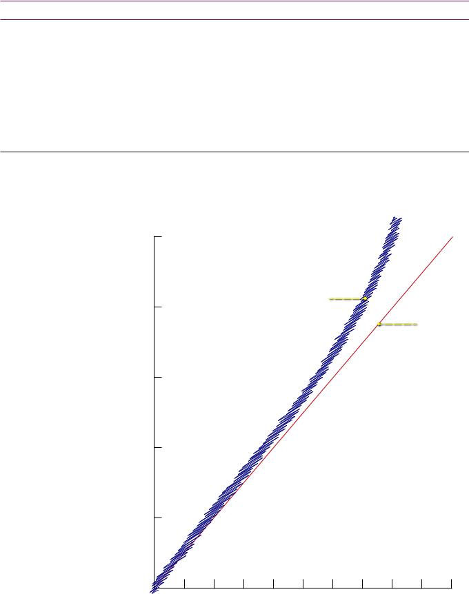
Nuclear medicine physics
Definitions |
A |
A = atomic mass = N + Z |
|
|
|
|
Z XN |
Z = # protons = atomic number |
|
N = # neutrons |
|
|
|
X = element |
•Isobar: Same atomic mass (e.g., 131I and 131Xe)
•IsotoPes: Same number of Protons
•IsotoNes: Same number of Neutrons
Decay and stability |
• The graph below demonstrates that as atomic number (Z) increases, stable |
|
elements tend to have slightly increased neutrons relative to protons. |
•Isotopes with excess neutrons decay by beta-minus decay, while isotopes with excess protons decay by beta-plus decay.
|
100 |
|
|
|
|
|
|
|
neutron excess |
|
|
|
|
|
|
β- decay |
|
|
|
|
|
80 |
|
|
band of |
|
|
|
|
|
stability |
|
|
|
|
|
|
|
|
|
N = Z |
(N) |
60 |
|
|
|
|
|
of neutrons |
|
|
|
|
|
|
|
|
|
|
proton excess |
||
number |
40 |
|
|
|
β+ decay |
|
|
|
|
|
|
||
|
|
|
|
|
|
|
|
20 |
|
|
|
|
|
|
0 |
20 |
40 |
60 |
80 |
100 |
number of protons (Z)
861

Alpha decay |
• An α particle is 2 protons and 2 neutrons = Helium nucleus |
•Alpha decay causes loss of an α particle: Atomic mass i by 4; Z i by 2 and N i 2
AZ –– 24 XN – 2
Beta minus decay |
• β– decay occurs with neutron excess: Neutron converted to proton. |
|
Z |
β−decay |
energy |
Z+1 |
|
|
|
|
|
Z (atomic number) |
|
•Elements produced in nuclear reactors are neutron rich.
Z +A1 XN – 1
Beta plus decay |
• β+ decay occurs with proton excess: Proton converted to neutron. |
Z |
energy |
Z-1 |
Z (atomic number)
β+ decay electron capture
•Elements produced in a cyclotron are proton-rich. β+ decay competes with electron capture (both cause Z i 1 and N h 1). Atomic mass is unchanged.
Z –A1 XN + 1
Electron capture |
• Electron capture is similar to, and competes with, β+ decay. A proton is |
|
converted to a neutron by capturing an e–, which usually comes from the |
|
K-shell. The resultant vacancy is filled by an outer shell e- and a characteristic |
|
X-ray or Auger e– is released. |
|
• The net change is identical to β+ decay: Z i 1 and N h 1, unchanged mass. |
|
• The following isotopes decay by electron capture (mnemonic: Cowboy says |
|
“GIIT over here” when trying to capture his horse): |
|
Gallium-67 |
|
Indium-111 |
|
Iodine-123 |
|
Thallium-201 |
862
Activity |
• |
The activity of a radionuclide is the number of decays per unit time. |
|
||||||||
|
• |
The activity at time (t) = N = N |
0 |
(e–λt) |
|
|
|
|
|
||
|
|
t |
|
|
|
|
|
|
|
||
|
|
N0 = initial activity |
|
|
|
|
|
|
|
|
|
|
|
Decay constant λ = 0.693/T½, where T½ = half life |
|
|
|
||||||
|
|
t = time elapsed |
|
|
|
|
|
|
|
|
|
|
|
|
|
|
|
|
|
||||
Cumulative activity |
• |
The cumulative activity is the total number of nuclear decays that occur over |
|
||||||||
|
|
time. It represents the area under the decay curve plotted over time. |
|
||||||||
|
• |
The cumulative activity = 1.44 x f x A0 x TE |
|
|
|
||||||
|
|
f = fractional uptake (assumed to be 1 if not explicitly stated otherwise) |
|
||||||||
|
|
A0 = initial activity |
|
|
|
|
|
|
|
|
|
|
|
TE = effective half-life |
|
|
|
|
|
|
|
|
|
|
|
|
|
|
|
|
|
||||
Effective half-life |
• |
The effective half-life is the half-life of a radionuclide within an organ, taking |
|
||||||||
|
|
into account the intrinsic physical half-life of the radionuclide and the biological |
|
||||||||
|
|
clearance. |
|
|
|
|
|
|
|
|
|
|
• |
The effective half-life = TE = |
|
1 |
|
= |
1 |
+ |
1 |
|
|
|
|
|
|
|
|
|
|
||||
|
|
|
|
TE |
|
TB |
T1/2 |
|
|||
|
|
TB = biologic half-life |
|
|
|
|
|
|
|
|
|
|
|
T1/2 = physical half-life |
|
|
|
|
|
|
|
|
|
|
|
|
|
||||||||
System resolution |
• |
System resolution is the resolution of the imaging system accounting for |
|
||||||||
|
|
the intrinsic resolution of the scintillation camera (without a collimator) and |
|
||||||||
|
|
resolution of the collimator. |
|
|
|
|
|
|
|
|
|
|
• |
System resolution = R = |
|
|
Ri2 + Rc2 |
|
|
|
|||
Ri = intrinsic resolution
Rc = collimator resolution
Quality control: |
• Constancy: Tested every day (“constantly”) with |
|
Dose calibrator |
|
137Cs (30 year half-life) |
|
• |
Linearity: Tested quarterly with 99mTc decay |
|
• |
Accuracy: Tested annually with a calibrated source |
•These are tests of the dose calibrator, not the imaging system!
Quality control: |
• Uniformity: Tested daily with Co-57 |
Imaging system |
|
863
References, resources, and further reading
Reference Textbooks:
Bushberg, J.T., Seibert, J.A., Leidholdt, E.M. & Boone, J.M. The Essential Physics of Medical Imaging (2nd ed.) Lippincott
Williams & Wilkins. (2001).
Huda, W. Review of Radiologic Physics (3rd ed.). Lippincott Williams & Wilkins. (2009).
Articles:
Bitar, R. et al. MR pulse sequences: what every radiologist wants to know but is afraid to ask. Radiographics, 26(2), 513-37(2006).
Cody, D.D. AAPM/RSNA physics tutorial for residents: topics in CT. Image processing in CT. Radiographics, 22(5), 1255-68(2002).
Cody, D.D. & Mahesh, M. AAPM/RSNA physics tutorial for residents: Technologic advances in multidetector CT with a focus on cardiac imaging. Radiographics, 27(6), 1829-37(2007).
Hedrick, W.R. & Mahesh, M. Radiation Biology for Diagnostic and Interventional Radiologists (5th ed.). Radiological Society of North America. (2007).
Jacobs, M.A., Ibrahim, T.S. & Ouwerkerk, R. AAPM/RSNA physics tutorials for residents: MR imaging: brief overview and emerging applications. Radiographics, 27(4), 1213-29(2007).
Mahesh, M. The AAPM/RSNA Physics Tutorial for Residents Fluoroscopy: Patient Radiation. Radiographics, 21, 1033-1045(2001).
Mahesh, M. AAPM/RSNA physics tutorial for residents: digital mammography: an overview. Radiographics, 24(6), 1747-60(2004).
McNitt-Gray, M.F. AAPM/RSNA Physics Tutorial for Residents: Topics in CT. Radiation dose in CT. Radiographics, 22(6), 1541-53(2002).
Mettler, F.A., Huda, W., Yoshizumi, T.T. & Mahesh, M. Effective doses in radiology and diagnostic nuclear medicine: a catalog. Radiology, 248(1), 254-63(2008).
Nickoloff, E.L., Lu, Z.F., Dutta, A.K. & So, J.C. Radiation dose descriptors: BERT, COD, DAP, and other strange creatures. Radiographics, 28(5), 1439-50(2008).
Pooley, R.A. AAPM/RSNA physics tutorial for residents: fundamental physics of MR imaging. Radiographics, 25(4), 1087-99(2005).
Schueler, B.A, Vrieze, T.J., Bjarnason, H. & Stanson, A.W. An investigation of operator exposure in interventional radiology. Radiographics, 26, 1533-41 (2006)., discussion 1541.
Zhuo, J. & Gullapalli, R.P. AAPM/RSNA physics tutorial for residents: MR artifacts, safety, and quality control. Radiographics, 26(1), 275-97(2006).
864