- •Contents at a glance
- •Contents
- •Introduction
- •Who this book is for
- •Assumptions about you
- •Organization of this book
- •Conventions
- •About the companion content
- •Acknowledgments
- •Errata and book support
- •We want to hear from you
- •Stay in touch
- •Chapter 1. Introduction to data modeling
- •Working with a single table
- •Introducing the data model
- •Introducing star schemas
- •Understanding the importance of naming objects
- •Conclusions
- •Chapter 2. Using header/detail tables
- •Introducing header/detail
- •Aggregating values from the header
- •Flattening header/detail
- •Conclusions
- •Chapter 3. Using multiple fact tables
- •Using denormalized fact tables
- •Filtering across dimensions
- •Understanding model ambiguity
- •Using orders and invoices
- •Calculating the total invoiced for the customer
- •Calculating the number of invoices that include the given order of the given customer
- •Calculating the amount of the order, if invoiced
- •Conclusions
- •Chapter 4. Working with date and time
- •Creating a date dimension
- •Understanding automatic time dimensions
- •Automatic time grouping in Excel
- •Automatic time grouping in Power BI Desktop
- •Using multiple date dimensions
- •Handling date and time
- •Time-intelligence calculations
- •Handling fiscal calendars
- •Computing with working days
- •Working days in a single country or region
- •Working with multiple countries or regions
- •Handling special periods of the year
- •Using non-overlapping periods
- •Periods relative to today
- •Using overlapping periods
- •Working with weekly calendars
- •Conclusions
- •Chapter 5. Tracking historical attributes
- •Introducing slowly changing dimensions
- •Using slowly changing dimensions
- •Loading slowly changing dimensions
- •Fixing granularity in the dimension
- •Fixing granularity in the fact table
- •Rapidly changing dimensions
- •Choosing the right modeling technique
- •Conclusions
- •Chapter 6. Using snapshots
- •Using data that you cannot aggregate over time
- •Aggregating snapshots
- •Understanding derived snapshots
- •Understanding the transition matrix
- •Conclusions
- •Chapter 7. Analyzing date and time intervals
- •Introduction to temporal data
- •Aggregating with simple intervals
- •Intervals crossing dates
- •Modeling working shifts and time shifting
- •Analyzing active events
- •Mixing different durations
- •Conclusions
- •Chapter 8. Many-to-many relationships
- •Introducing many-to-many relationships
- •Understanding the bidirectional pattern
- •Understanding non-additivity
- •Cascading many-to-many
- •Temporal many-to-many
- •Reallocating factors and percentages
- •Materializing many-to-many
- •Using the fact tables as a bridge
- •Performance considerations
- •Conclusions
- •Chapter 9. Working with different granularity
- •Introduction to granularity
- •Relationships at different granularity
- •Analyzing budget data
- •Using DAX code to move filters
- •Filtering through relationships
- •Hiding values at the wrong granularity
- •Allocating values at a higher granularity
- •Conclusions
- •Chapter 10. Segmentation data models
- •Computing multiple-column relationships
- •Computing static segmentation
- •Using dynamic segmentation
- •Understanding the power of calculated columns: ABC analysis
- •Conclusions
- •Chapter 11. Working with multiple currencies
- •Understanding different scenarios
- •Multiple source currencies, single reporting currency
- •Single source currency, multiple reporting currencies
- •Multiple source currencies, multiple reporting currencies
- •Conclusions
- •Appendix A. Data modeling 101
- •Tables
- •Data types
- •Relationships
- •Filtering and cross-filtering
- •Different types of models
- •Star schema
- •Snowflake schema
- •Models with bridge tables
- •Measures and additivity
- •Additive measures
- •Non-additive measures
- •Semi-additive measures
- •Index
- •Code Snippets
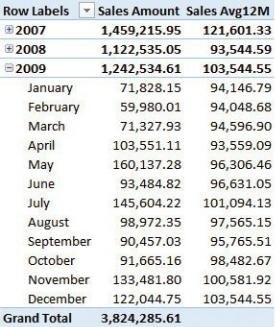
FIGURE 4-20 The measure computes the average over 12 months.
Handling fiscal calendars
Another very good reason you should create your own Calendar table is that it makes it very easy to work with a fiscal calendar. Alternatively, in more extreme situations, you can work with more complex calendars, like weekly or seasonal calendars.
When handling a fiscal calendar, you do not need to add additional columns to your fact table. Instead, you simply add a set of columns to your Date table so that you will be able to slice by using both the standard and the fiscal calendar. As an example, imagine you need to handle a fiscal calendar that sets the first month of the year as July. Thus, the calendar goes from July 1st to June 30th. In such a scenario, you need to modify the calendar so that it shows fiscal months, and you will need to modify some calculations to make them work with fiscal calendars.
First, you need to add a suitable set of columns to hold the fiscal months (if they are not yet there already). Some people prefer to see July as the name of the first fiscal month, whereas other people prefer to avoid month names and use numbers instead. Thus, by using numbers, they browse the month as Fiscal Month 01 instead of July. For this example, we use the standard names for months.
No matter which naming technique you prefer, for proper sorting, you will need an additional column to hold the fiscal month name. In standard calendars, you have a Month Name column, which is sorted by Month Number, so that January is
put in the first place and December in the last place. In contrast, when using the fiscal calendar, you want to put July as the first month and June as the last one. Because you cannot sort the same column using different sorters, you will need to replicate the month name in a new column, Fiscal Month, and create a new sort column that sorts the fiscal month the way you want.
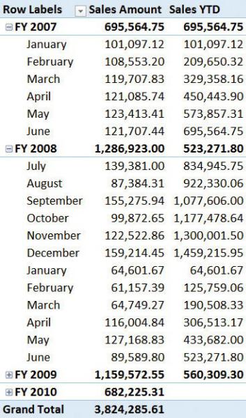
After these steps are done, you can browse the model using columns in your Calendar table, and you can have the months sorted the right way. Nevertheless, some calculations will not work as expected. For example, look at the Sales YTD calculation in the PivotTable shown in Figure 4-21.
FIGURE 4-21 The YTD calculation does not work correctly with the fiscal
calendar.
If you look carefully at the PivotTable, you can see that the value of YTD is reset in January 2008 instead of July. This is because the standard timeintelligence functions are designed to work with standard calendars, and because of that, they do not work with custom calendars. Some functions have an additional parameter that can instruct them on how to work with fiscal calendars. DATESYTD, the function used to compute YTD, is among them. To compute YTD with a fiscal calendar, you can add a second parameter to DATESYTD that specifies the day and month at which the calendar ends, like in the following code:
Click here to view code image
Sales YTD Fiscal := CALCULATE (
[Sales Amount],
DATESYTD ( 'Date'[Date], "06/30" )
)
Figure 4-22 shows the PivotTable with the standard YTD and the fiscal YTD, side-by-side.
FIGURE 4-22 Sales YTD Fiscal resets correctly, at the end of July.
Obviously, different calculations might require different approaches, but the standard timeintelligence functions provided in DAX can be easily adapted to fiscal calendars. In the last section of this chapter we will cover weekly calendars, which are another useful variation on calendars. If you have different needs, or if you need to work with even more complex calendars, then you need to follow a more complex approach; we suggest you look at the time-intelligence patterns at http://www.daxpatterns.com/time-patterns/.
The important point for the sake of this book is that you do not need additional tables to handle fiscal calendars in a smooth way. If your Date table is designed