Добавил:

mihail1000 Опубликованный материал нарушает ваши авторские права? Сообщите нам.

Вуз:

Воронежский государственный технический университет

Предмет:

[НЕСОРТИРОВАННОЕ]

Файл:

Учебное пособие 2132

.pdf

Скачиваний:

Добавлен:

30.04.2022

Размер:

6.9 Mб

Скачать

☆

<<< < Предыдущая 1 2 34 / 114 5 6 7 8 9 10 11 > Следующая >>>

Russian Journal of Building Construction and Architecture

Thus

ln| x|*q(x) l (x)

q(y)ln

x y

dly.

(3.6)

Similarly (3.6) we find that

q(x) l

(x)

q(y)

x y

dly .

(3.7)

2 l

From (3.1), (3.2), (3.6) and (3.7) we get

(y )

q1(y)ln

uˆ(x)

dy1

x y

dly

1(y)ln

x y

dly

x )2 x2

(3.8)

x y

(y)

dly

(y)

dly.

In (2.4) and (2.5) it was noted that at

x (x1,x2 ) l

(x) q

(x ,x ) q (x , x );q

(x) q (x , x ).

Considering the two last equalities (3.8) we get the following

u(x)

(y )

q1(y) ln| x y| ln| x y | dly

dy1

y )2

(3.9)

ln| x y|

ln| x y

q0 (y)

dly ,

where

( sin ;cos ),

( sin ; cos ), y (y1,y2), y

(y1, y2).

4. Prove of mathematical correctness of the model. Formula for presenting the solution of the model. Note that at this stage we cannot argue that the function u(x)is the solution of the task (1.1)––(1.4) as it was obtained assuming that the task (1.1)––(1.4) is correct (that it has the solution). Let us prove that the functionu(x) given by the equality (3.9) under the

previously stated conditions in the function (x1),

q0 (x), q1(x)

will be the solution of the

task (1.1)––(1.4), i.e. the solution of the task (1.1)––(1.4) is given by the formula:

(y )

q1(y) ln| x y| ln| x y | dly

u(x)

dy1

(x y )2 x2

(4.1)

ln| x y|

ln| x y |

(y)

dly ,

where n ( sin ;cos ),n1 ( sin ; cos ), y (y1,y2), y (y1, y2).

Issue № 2 (42), 2019

ISSN 2542-0526

In [4] it was shown that if the function f (x)is continuous in the entire real line probably except a finite number of points where it has the discontinuity of the first kind, for any number of 0 the following ratio holds true:

	x1		f (y )			f (x 0) f (x 0)
lim			1		dy	1	1	,	(4.2)
lim			(x y )2	2	dy		2	,	(4.2)
0			(x y )2	2	1		2
		x	1 1
		1

where f (x1	0) lim	f (x1	), f (x1	0) lim	f (x1 ).
	0			0

Let us show that the functionu(x)given by the equation (4.1) meets the conditions (1.2). It is plain to see that

u(x1 lim u(x1,x2)

x2 0

lim

(y )

dy lim

q (y)

ln| x y| ln| x y

x2 0

y1)

x2 0

(x1

2 l

lim

q (y)

ln|

x2 0

n1x

2 l

The restrictions of the function (x1)

and (4.2) mean that

lim

(y )

lim

(y )

x 0

(x1

y1)

(x1 y1)

lim

(y )

dy lim

(y )

(x1

y1)2 x22

x (x1 y1)2 x22

x2 0 x

x2 0

lim

x x1

(y )

dy (x ).

x2 0 x (x1 y1)2 x22

It is plain to see that

lim

q (y)

ln| x y| ln| x y

2 l

q (y) lim

ln| x y| ln| x y

x2 0

2 l

q1(y)(ln

(x1 y1)

( y2 )

(x1 y1)

y2 dly

It is plain to see that

lim

q (y)

ln|

y |

n1x

q (y) lim

ln|

x 0

n1x

(4.3)

(4.4)

(4.5)

(4.6)

Russian Journal of Building Construction and Architecture

Using (4.3)––(4.6) we find that

u(x1 lim u(x1,x2) (x1) ,

x2 0

i.e. the condition (1.2) is met.

Similarly using (4.2) we see that for the functionu(x)given by the equation (4.1), the conditions (1.3), (1.4) are met.

Immediately inserting the functionu(x)into the equation (1.1) we make sure that it is its solution.

Conclusions. The paper looked into essential and urgent research issues related to mathematical description of heat distribution in defected materials and structures as well as determining how defects in materials and structures influence the temperature of materials and structures. A mathematical model is suggested that allows the temperature distribution to be identified in the half plane with a rectangular crack reaching the half plane boundary knowing the temperature at the half plane boundary and fluctuations of temperature and heat flows in the crack. Using the methods of the theory of generalized functions mathematical correctness of the model was proved and the formula the solution is given by was obtained.

The resulting formula can be used for analyzing the behavior of the temperature in material with a crack including for identifying singularities in the adjacent areas as well as the effect of cracking on heat distribution. Note that the first of the summands in the formula of presenting the solution shows the temperature in the half plane with no cracking if the temperature at the boundary of the half plane is known while the formula itself can be generalized for a random smooth crack.

References

1.Vladimirov V. S. Uravneniya matematicheskoi fiziki [Equations of mathematical physics]. Moscow, Nauka Publ., 1976. 527 p.

2.Vladimirov V. S. , Mikhailov V. P., Vasharin A. A. e. a. Sbornik zadach po uravneniyam matematicheskoi fiziki [Collection of problems on equations of mathematical physics]. Moscow, Nauka Publ., 1982. 256 p.

3.Glushko A. V., Ryabenko A. S., Loginova E. A., Petrova V. E. Izuchenie statsionarnogo raspredelenie tepla v ploskosti s treshchinoi pri peremen-nom koeffitsiente vnutrennei teploprovodnosti [Study of stationary heat distribution in a plane with a crack at a variable coefficient of internal thermal conductivity]. Zhurnal vychislitel'noi matematiki i matematicheskoi fiziki, 2015, vol. 55, no. 4, pp. 695––703.

4.Glushko A. V., Ryabenko A. S., Chernikova A. S. O statsionarnom raspredelenii tepla v dvukh svyaznykh poluploskostyakh s treshchinoi na granitse [On stationary heat distribution in two connected half-planes with a crack at the boundary]. Vestnik VGU. Seriya. Fizika. Matematika, 2015, no. 1, pp. 111––134.

Issue № 2 (42), 2019

ISSN 2542-0526

5.Ordyan M. G., Petrova V. E. Zadacha teploprovodnosti dlya bimateriala s sistemoi chastichno teplopronitsaemykh treshchin i teplovym istochnikom [The problem of thermal conductivity for bimaterial with a system of partially heat-permeable cracks and a heat source]. Vestnik Samarskogo gosudarstvennogo univer-siteta (Estestvennonauchnaya seriya), 2009, no. 4 (70), pp. 154––170.

6.Panasyuk, V. V., Savruk M. P., Datsyshin A. P. Raspredelenie napryazhenii okolo treshchiny v plastinakh i obolochkakh [Distribution of stresses around cracks in plates and shells], Kiev, Nauk. Dumka Publ., 1976. 445 p.

7.Parton V. Z. Mekhanika razrusheniya [Fracture mechanics], Moscow, Nauka Publ., 1990. 240 p.

8.Ryabenko A. S. Asimptoticheskie svoistva resheniya zadachi o statsionarnom raspredelenii tepla v odnorodnoi ploskosti s treshchinoi [Asymptotic properties of the solution of the problem of stationary heat distribution in a homogeneous plane with a crack]. Vestnik VGU. Seriya. Fizika. Matematika, 2012, no. 1, pp. 187––194.

9.Ryabenko A. S. O statsionarnom raspredelenii tepla v funktsional'no-gradientnykh materialakh s vnutrennei treshchinoi [On stationary heat distribution in functionally graded materials with internal crack]. Vestnik Voronezhskogo instituta GPS MChS Rossii, 2014, vol. 2, pp. 40––45.

10.Ryabenko A. S., Chernikova A. S. O edinstvennosti resheniya zadachi, modeliruyushchei raspredelenie tepla v ploskosti s treshchinoi na styke dvukh materialov [On the uniqueness of the solution of the problem modeling the heat distribution in the plane with a crack at the junction of two materials]. Vestnik VGU. Seriya. Fizika. Matematika, 2017, no. 4, pp. 124––133.

11.Chiu Tz-Cheng, Tsai Shang-Wu, Chue Ching-Hwei. Heat conduction in a functionally graded medium with an arbitrarily oriented crack. International Journal of Heat and Mass Transfer, 2013, vol. 67, pp. 514––522.

12.Erdogan F. The crack problem for bonded nonhomogeneous materials under antiplane shear loading. J. Appl. Mech, 1985, vol. 52, pp. 823––828.

13.Glushko A. V., Ryabenko A. S., Petrova V. E., Loginova E. A. Heat distribution in a plane with a crack with a variable coefficient of thermal conductivity. Asymptotic Analysis, 2016, vol. 98, no. 4, pp. 285––307.

14.Lee K. Y., Shul C. W. Determination of the thermal stress intensityfactors for an interface crack under vertical uniform heat flow. Eng. Fract. Mech, 1991, vol. 40, no. 6, pp. 1067––1074.

15.Lee K. Y., Park S. J. Thermal stress intensity factors for partially insulated interface crack under uniform heat flow. Eng. Fract. Mech, 1995, vol. 50, no. 4, pp. 475––482.

16.Petrova V., Schauder S. Thermal fracture of a functionally graded/homogeneous bimaterial with a system of cracks. Teoretical and Applied Fracture Mechanics, 2011, vol. 55, pp. 148––157.

17.Sladek J., Sladek V., Zhan Ch. An advanced numerical method for computing elastodyanamic fracture parameters in functionallygraded materials. Computational Materials Science, 2005, vol. 32, pp. 532––543.

18.Wang X. D., Meguid S. A. The interaction between an interfacial crack and a microcrack under antiplane loading. International Journal of Fracture, 1996, vol. 76, pp. 263––278.

Russian Journal of Building Construction and Architecture

DESIGNING AND CONSTRUCTION OF ROADS, SUBWAYS,

AIRFIELDS, BRIDGES AND TRANSPORT TUNNELS

DOI 10.25987/VSTU.2019.42.2.004

UDC625.7.004:551.58

V. A. Kozlov1, A. I. Kotov2, A. V. Loboda3

MODELLING FAILURES OF ASPHALT CONCRETE SURFACINGS

CAUSED BY A DYNAMIC IMPACT OF WATER

Voronezh State Technical University

Russia, Voronezh

1D. Sc. in Physics and Mathematics, Head of the Dept. of Theoretical and Applied Mechanics, tel.: (473)276-40-06, e-mail: v.a.kozlov1@yandex.ru

3D. Sc. in Physics and Mathematics, Prof. of the Dept. of Applied Mathematics and Mechanics, tel.: (473)271-53-62, e-mail: lobvgasu@yandex.ru

Research Centre «Zhukovsky-Gagarin Air Force Academy»

Russia, Voronezh

2Junior Research Fellow of the 24th Research Department of the Scientific,

tel.: 8-910-240-25-87, e-mail: kotlac@yandex.ru

Statement of the problem. The central factor contributing to road failures is a dynamic impact of traffic. An asphalt surfacing is mainly dry, but when it gets wet, there is frequently an increase in the number of defects. The methods and ways of determining the defect growth rate in dry roads provide insight into the mechanisms of development of defects and ways to enhance the longevity and defect resistance of asphalt concrete.

Results. We present modeling of a dynamic impact of water on asphalt concrete surfacing and provide the methods of measuring it under a traffic load. Calculations of changes in the pressure inside pores of the upper layer of a surfacing and water speed in spots where defects emerge are shown. Aconnection was found between theparameters ofa traffic flow and defects occurring in a surfacing.

Conclusions. We found that besides the known and described defects a roadway surfacing might fail due to an impact of wheels provided there is some water on the surface (water wear and tear). A dynamic impact of water moving under a rolling wheel of a vehicle on an asphalt concrete surfacing is complex and modeling it involves analysis of the structure of asphalt concrete.

Keywords: wear and tear of roadwaysurfacings, asphalt concrete surfacing, dynamic impact of water.

Introduction. Highway roadways tend to develop plastic deformations, ruts, heaving, etc. [2]

with long-term operation invariably resulting in intensive wear and tear. At the modern

Issue № 2 (42), 2019

ISSN 2542-0526

development stage the properties of roadway materials are being improved but asphalt concrete strength always remains an issue.

The article looks at water circulation and modeling its movement in the upper layer of a roadway under the impact of vehicle wheels. As a result, pressure fields and water velocities in asphalt concrete pores have been deisgned that cause extra strains leading to defects in a roadway.

1. Statement of the problem. Impact of load on a road structure has been investigated by scientists in this country and abroad (e.g., see [2, 13, 14]) which revealed a correlation between a static and dynamic load impact on plastic deformation and wear and tear. According to the analysis of highways, one of the most common defects on non-rigid roadways is rut. The way defects are formed into ruts on the surface of an asphalt concrete roadway under a traffic impact in a variety of operating conditions has not been studied in its entirety and is underpinned with complex dependencies, which is caused by different effects, i.e. plastic deformation, wear and tear including deformation of the foundation. It is noted that wherever traffic is particularly intense, irreversible deformations of an asphalt concrete roadway and traffic flow characteristics are connected causing ruts. The geometric parameters of ruts can vary significantly depending on the impact. Modern scientific and regulative literature suggests that while assessing a roadway dynamic water impact on an asphalt concrete roadway giving rise to extra rutting is not completely accounted for.

One of wears of a roadway surface is micropores and cracks where water starts circulating if moisted. Existing methods do not allow this circulation to be measured and its impact on the stress-strain of the upper layer of asphalt concrete to be evaluated and thus a resulting wear and tear caused by traffic to be taken into consideration. In [4, 6] there are mechanisms of wear and tear during dry friction. The authors indicate how uneven this wear and tear is in different operational periods without specifying the reasons therefor. The connection they designed between the intensity and scope of wear and tear has no correlation with whether this is a city or a small road. Studies of transport impact on roadways for superficial moisture also allows one to assume there might be failures of asphalt concrete roadways caused by other physical processes [5]. According to the analysis of research related to tribomechanical impact of moving rollers along asphalt concrete samples, there are extra interactions occurring in the contact of a roller. Moisturizing the samples causes them to change resulting in extra power losses. This allows one to assume that moisture influences a wheel-roadway contact. Wear and tear obviously occurs in the contact and causes failure of the upper elements of a

Russian Journal of Building Construction and Architecture

roadway under the impact of water inside it. The impact of the wheel on the contact with tangential and normal stresses might result in cracks and pore opening. Moisture stimulates filling of pores and according to [1], this might lead to a hydraulic effect from the impact of an elastic rubber on the roadway surface accompanied by defects. In order to allow for and analyze the effect, it is necessary to calculate the resulting contact of the wheel with the pressure surface inside the water-filled pores.

2. Equations of the model of water movement in the pores of the upper layer of a road-

way surface. A few factors [2, 3, 9, 13] contribute to the above defect of an asphalt concrete surfacing. In order to evaluate the influence of each of the factors causing rutting by means of the waterjet effect, a series of theoretical studies and modeling was performed to enable us to group the influence of the various factors on abrasive ruts in the dry as well as wet condition. Studying deformations in parts of non-rigid roadways with an asphalt concrete surfacing under the traffic impact called for an original method of evaluating the effect of dynamic impact of traffic on a dry asphalt concrete roadway surfacing.

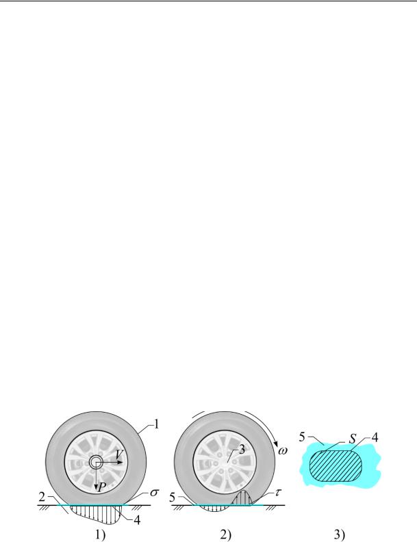
Traffic along the surfacing causes an intense water flow and dynamic compression under the “pneumatics –– water –– roadway” contact area. Due to poor compressibility water starts moving at an increasing speed. The modeling showed that at the moment the tangential stresses in the surface dropped the rate of a water flow from under the front of the contact might increase two-fold and the liquid pressure in the contact area is comparable with that in the wheel pneumatics (Fig. 1).

Fig. 1. Distribution of normal and tangential stresses in the surfacing under the wheel for a drycondition of the surfacing:

1 is a vehicle wheel; 2 is a roadwaysurfacing; 3 is a vehicle axis; 4 is a wheel imprint; 5 is a moistened area of the surfacing

Issue № 2 (42), 2019

ISSN 2542-0526

The solution involves the operation of the wheel along the surface. Let us assume that a vehicle is a reciprocating coordinate system [1] with a positive movement towards the front of the incoming part of the tire. In this case the bending w is described with a differential equation

T v2	d2w	k1	dw	kw Q,	(1)
	2
	ds		ds

where Т is a stretching effort in the pneumatics; k is the rigidity of the elastic foundation; µ is the massunit ofthe length;v isthe rolling speed;the coefficientk1 describes attenuation. Inorderto determine the bending inthe model, let usdescribe the initialpositionusing a homogeneousequation:

T v 2	d2w	k	dw	kw 0,	(2)
	ds2
		1	ds

whose particular solution can be presented as w = ecs. By substituting and reducing it by ecs, we get a quadratic equation in relation to the coefficient с:

T – µv2 с2 k1с –k 0.

(3)

As long as the rolling speed v is small, с1 is negative and с2 is positive and thus the equation

(3) has two solutions, i.e. the one that goes down as the curve s increases: w1 Aec1s and goes up as it does so as well: w2 Bec2 s where А and В are constants of a free part of the model and contact area. It is obvious that the increasing part of the wheel at

T vкр µ

remains undeformed and the impact on the surface is mechanical movement of the wave along the tire. If the rolling speed is more than vkp, the ring material moves faster than the deformations generated by loads applied to the contact area propagate.

It should be noted that rolling of the wheel at the speed more than vkp leads to the concentrated impact force Pj that can be easily determined considering changes in the amount of traffic at the contact entry. Every time over the time dt this area moves into a new position causing the vertical component of the amount of its traffic to drop by μvdtsinφ. The vertical projection of the impulse of the forces applied to the area over the same amount of time is (Pj + Tsinφ)dt.

Expressing the change in the amount of traffic proportionate to the force impulse we find

Pj v2 T sin .

sin 2w ,

Russian Journal of Building Construction and Architecture

ultimately we get:


	v2		fw
P		1 2		.	(4)

j	v2		R
	кр

The impact force Pj yields a moment in relation to the axis


			v2
M	j	Pa T		1 2w.	(5)
M		Pa T		1 2w.	(5)
		j	v2
			кр

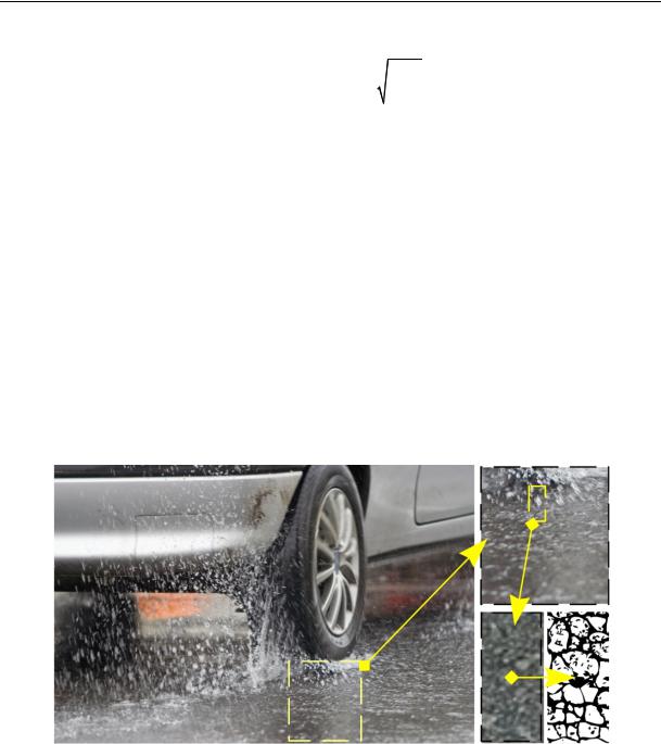
3. Results of the numerical modeling. An area of the asphalt concrete surfacing in the immediate vicinity to the wheel is used for modeling and the surface of the area is covered with a thin layer of a liquid penetrating its pores and cracks. The modeled element is 10 mm in length and 20 mm in width. The volume of the liquid is proportionate to that of the open pores and cracks in the element. A vehicle travels at the speed of 10 m/sec and hits the element with its wheel blocking the upper part of the pore with the wheel rubber with the pressure in the pneumatics 2×105 Pа (Fig. 2).

Fig. 2. Modelling area of the wheel impact on the moistened surfacing

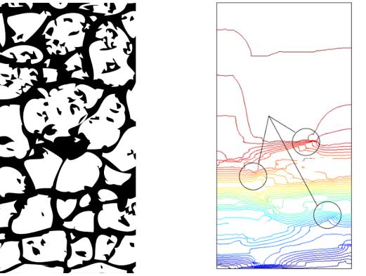
As a result of loading the liquid in the pores starts moving coming into the depth of a defected area. Fig. 3b shows the distribution of the pressure under the impact of a vehicle wheel. Pressure isolines indicate changes in its depth accompanied with uneven distribution as under the influence of an external wheel load the material also sets in motion once there is a local zone of a higher pressure gradient. It is obvious that when there is no more load, the pressure strives to expand the material particles causing their hydraulic breakage. According to calcu-

Issue № 2 (42), 2019

ISSN 2542-0526

lations, there might be a pressure difference within a millimetre’s distance inside the layer under the specified load P = 0.4––1.0 atmospheres, which might be greater than the bitumen adhesion of the mineral component.

The analysis of the results showed that an increase in the bending of a road structure under a traffic influence compared to a single vehicle generates large bends causing more intense wear and tear. An increase in the speed of a vehicle generates a greater “dry” wear and tear. As it moves along a wet surfacing of the wheel, it is affected by the hydrodynamic elevating force that reduces the friction of the material on the road.

а)

1,98×105 Pa

Large pressure

gradient

1,7×105 Pa

1,01×105 Pa

Fig. 3. Structure of a cut of a failure of an asphalt concrete surfacing with micropores which is its digital image:

а) the cavities filled with water are in black and the mineral and bitumen material

of asphalt concrete is colourless; b) graph of pressure level lines emerging in the channels with the liquid and equivalent pressure acting on the material

Further modeling suggests that a growth in P as a non-linear dependence on the tire pressure of a vehicle and its speed. Fig. 4 shows the graphs of the dependence of the maximum pressure inside a roadway element experiencing failture and pressure gradient on the speed of a

<<< < Предыдущая 1 2 34 / 114 5 6 7 8 9 10 11 > Следующая >>>

Соседние файлы в предмете [НЕСОРТИРОВАННОЕ]

#
30.04.20226.82 Mб8Учебное пособие 2128.pdf
#
30.04.20226.82 Mб3Учебное пособие 2129.pdf
#
30.04.2022330.75 Кб2Учебное пособие 213.pdf
#
30.04.20226.87 Mб27Учебное пособие 2130.pdf
#
30.04.20226.89 Mб1Учебное пособие 2131.pdf
#
30.04.20226.9 Mб1Учебное пособие 2132.pdf
#
30.04.20226.92 Mб9Учебное пособие 2133.pdf
#
30.04.20226.98 Mб2Учебное пособие 2134.pdf
#
30.04.20227.13 Mб3Учебное пособие 2135.pdf
#
30.04.20227.14 Mб9Учебное пособие 2136.pdf
#
30.04.20227.26 Mб7Учебное пособие 2137.pdf