Учебное пособие 2132

Russian Journal of Building Construction and Architecture

Let us look at the temperature at the cooler output Tk( ) in more detail. The papers [8, 10, 12, 14, 18] dealt with physical processes in indirect evaporative air coolers. As the the humidity level of the air remains the same, the temperature can be determined using a mathematical model of heat and mass transfer [6, 7, 21, 22] in recuperative indirect evaporative coolers.

Heat transfer in the channel s of the recuperative cooler is described using the parabolic equations (see Fig. 2):

y

Fig. 2. Section of the evaporative nozzle

Equation of heat and mass transfer in the “wet” channel is the following:

The temperature in the plate is distributed according to the Laplace law:

10

The input conditions are as follows:

In the axis of the channel s there is a symmetry condition:

The faces of the plates are modeled as being heat resistant:

In addition, the conditions of joining the temperature and heat fluxs are specified:

According to [3, 4, 23], the diffusion coefficient D, m2/seс is assumed to be zero

D 10 5 2.16 1 t / 273 1.8 .

The density of the saturation of the water vapourwн t , kg/m3, is given by the formula:

wн t 0.0004212t3 0.001831t2 0.4195t 4.727 10 3 ,

approximating the table data [3]. Here W is the density of the vapour, kg/m3, λпл, ρ, С is the heat conchannel ivity of the plate, Watt/m/degrees, the air density, kg/m3 and the specific heat capacity, J/kg/degrees, R(t) (2500.6 2.372t) 103 is the specific heat of vapour formation, J/kg, ε is a multiplier of an energy supplement considering the property of the evaporative porous surfaces.

3. Implementation of the mathematical model. As heat and mass transfer in the cooling block is described by different types of equations in particular derivatives, the section of the plate as well as that of the channel s are split by a rectangular grid that is made up by the finite difference analogues of the components of the above model of equations [5, 7, 10].

11

Russian Journal of Building Construction and Architecture

The resulting system of linear algebraic equations is solved for the density of the saturated vapour and the coefficients of heat conductivity and diffusion calculated for the initial air temperature in the facility. Then the density of the saturated air and the above coefficients are corrected depending on the resulting temperatures and the system is solved again. Iteration stops when the temperature in the previous and current iterations at the cooler output differ not more than by 0.1 0С.

Changes in the temperature at the output of the recuperative indirect cooler at different temperatures of the input air with a constant humidity level of 19.75 g/kg of air are given in Table.

Таble

Тemperature of the main air flux at the output of the recuperative cooler at different temperatures of the incoming air with a constant humiditylevel

The dependence of the temperature at the cooler output at a constant humidity level of 19.75 g/kg of air is given in Fig. 2. In this case the dependence of the output temperature on the input one is as follows: Тk = 0.2445T + 16.24. This temperature can be inserted into (1).

Fig. 4 presents a graph of the dependence of the air temperature in the cooling facility with technological equipment sized 6m × 6m× 3m. The heat emissions of the equipment are 40 kWatt, the initial temperature in the facility is modeled as being 380С, the temperature of the surface of the enclosure 200С, the consumption of the main air flux is 16000 cubic m/h, the consumption of the auxiliary air flux is 8000 cubic m/h. As the graph shows, the air temperature in the facility drops quickly and then rises as the enclosing surfaces are heated and reaches 26.40С.

12

Fig. 3. Graph of the dependence of the output temperature on the input one at a constant humiditylevel of 19.75 g/kg of air

Fig. 4. Graph of the dependence of the temperature in the cooling facilityon time

Conclusions

1.The mathematical model of heat balance of the underground facility with large heat emissions of the equipment cooled by evaporative air coolers is proposed.

2.The mathematical model of the heat and mass transfer in indirect evaporative recuperative coolers was also suggested that includes the temperature distribution equation in the plates of the evaporative nozzle that allows proper consideration to be given to their longitudinal and transverse heat conchannel ivity.

13

Russian Journal of Building Construction and Architecture

3.As a result of the research, we found that indirect recuperative evaporative coolers allow the temperature in facilities with technological equipment emitting a great deal of heat to be reduced without increasing the air humidity level.

4.Thesuggested mathematical model of thermal and physical processes in the heat exchangechannel s and its implementation methods enable the geometric parameters and operating modes of cooling blocks to be determined, which is applicable in engineering calculations.

5.Heat balance of the facility in question that gives consideration to the semi-infinite enclosing surface allows the performance of the indirect evaporative recuperative coolers to be evaluated in different operating modes and track the dynamics of temperature change of air environment over time.

6.The calculations proved the setups efficient to use with their environmental friendliness and costeffectiveness adding to the advantages they offer. Besides, a similar approach could be employed in the coolers operating in accordance with the Maisotsenko (M) cycle [11, 13, 16, 17, 19, 20].

References

1.Anisimov S. M., Pandelidis D., Polushkin V. I. Vliyanie parametrov naruzhnogo vozdukha na effektivnost' raboty perekrestno-tochnogo teploobmennika kosvenno-isparitel'nogo tipa [Influence of outdoor air parameters on the efficiency of the cross-accurate indirect-evaporative heat exchanger]. Vestnik grazhdanskikh inzhenerov, 2012, no. 4 (33), pp. 179––187.

2.Arkhiptsev A. V., Ignatkin I. Yu., Kuryachii M. G. Effektivnaya sistema ventilyatsii [Effective ventilation system]. Vestnik NGIEI, 2013, no. 8 (27), pp. 10––15.

3.Garanov S. A., Zharov A. A., Panteev D. A., Sokolik A. N.Vodoisparitel'noe i kombinirovannoe okhlazhdenie vozdukha [Water evaporation and combined air cooling]. Inzhenernyi zhurnal: nauka i innovatsii, 2013, no. 1 (13), p. 40.

4.Emel'yanov A. L., Gorbatov K. M., Garanov S. A. Gibridnaya isparitel'no-kompressionnaya ustanovka konditsionirovaniya vozdukha [A hybrid evaporation-compression air conditioning plant]. Vestnik Mezhdunarodnoi akademii kholoda, 2013, no. 4, pp. 34––37.

5.Ignatkin I. Yu. Matematicheskaya model' vodoisparitel'nogo okhlazhdeniya s oroshaemymi poverkhnostyami [A mathematical model photospreteen cooling with the irrigated surfaces]. Vestnik NGIEI, 2016, no. 6 (61), pp. 23––30.

6.Ignatkin I. Yu., Kirsanov V. V. Universal'naya ustanovka obespecheniya mikroklimata [Universal installation of providing a microclimate]. Vestnik NGIEI, 2016, no. 8 (63), pp. 110––116.

7.Ignatkin I. Yu. Sposob utilizatsii teploty vytyazhnogo vozdukha s primeneniem rekuperativnogo teploobmennika [Method of heat recovery of exhaust air with the use of recuperative heat exchanger]. Vestnik Voronezhskogo gosudarstvennogo agrarnogo universiteta, 2018, no. 1 (56), pp. 143––148.

8.Barakov A. V., Dubanin V. Yu., Prutskikh D. A., Naumov A. M. Issledovanie vozdukhookhladitelya kosvenno-isparitel'nogo tipa s dispersnoi nasadkoi [Investigation of air cooler of indirect-evaporative type with dispersed nozzle]. Promyshlennaya energetika, 2010, no. 11, pp. 37––40.

14

9. Kuz'min M. S. Povyshenie effektivnosti raboty draikulerov pri intensifikatsii protsessa teplootdachi [Improving the efficiency of the drycoolers take off at the intensification of the process of heat transfer].

Energobezopasnost' i energosberezhenie, 2015, no. 4, pp. 8––11.

10.Kuz'min M. S. Energosberezhenie pri intensifikatsii teploobmena v sistemakh konditsionirovaniya zdanii [Energy saving in the intensification of heat exchange in air conditioning systems of buildings]. Academia. Arkhitektura i stroitel'stvo, 2015, no. 2, pp. 120––124.

11.Osipov E. N. [Modeling of physical processes in indirect-recuperative water evaporative coolers]. Trudy “Nauka i obrazovanie v sovremennykh usloviyakh” [Proc. of the scientific conference "Science and education in modern conditions»]. Voronezh, VGAU Publ., 2016, pp. 117––124.

12.Terekhov V. I., Gorbachev M. V., Kkhafadzhi Kh. K. Optimizatsiya parametrov kosvenno-isparitel'nykh yacheek pri sputnom i vstrechnom techenii teplonositelei [Optimization of parameters of indirect-evaporative cells at satellite and counter-flow of heat carriers]. Teplovye protsessy v tekhnike, 2016, no. 5, pp. 207––213.

13.Shatskii V. P., Gulevskii V. A. Modelirovanie raboty plastinchatykh vodoisparitel'nykh okhladitelei kosvennogo printsipa deistviya [Modeling of the plate photospreteen coolers indirect principle].

Lesotekhnicheskii zhurnal, 2013, no. 4 (12), pp. 160––166.

14.Anisimov S., Pandelidis D. Numerical Study of the Maisotsenko Cycle Heat and Mass Exchanger. International Journal of Heat and Mass Transfer, 2014, vol. 75, pp. 75––96.

15.Chengqin R., Hongxing Y. An Analytical Model for the Heat and Mass Transfer Processes in Indirect Evaporative Cooling with Parallel/Counter Flow Configurations. International Journal of Heat and Mass Transfer, 2006, vol. 49, no. 3, pp. 617–627.

16.Duan Z., Zhan C., Zhang X., Mustafa M., Zhao X., Alimohammadisagvand B., Hasan A. Indirect Evaporative Cooling: Past, Present and Future Potentials. Renewable and Sustainable Energy, 2012, vol. 16, pp. 6823–– 6850.

17.Fakhrabadi F., Kowsary F. Optimal Design of a Regenerative Heat and Mass Exchanger for Indirect Evaporative Cooling. Applied Thermal Engineering, 2016, vol. 102, pp. 1384––1394.

18.Heidarineiad G., Bozorgmehr M. Heat and Mass Transfer Modeling of Two Stage Indirect/Direct Evaporative Aircoolers. ASHRAE Thailand Chapter Journal, 2007––2008, vol. 1, pp. 2––8.

19.Hutter G. W. The Status of World Geothermal Power Generation. Proc. of the World Geothermal Congress. Kyushu-Tohoku, 2000, pp. 23––37.

20.Kandlikar S. G., Garimella S., Li D., King M. R. Heat Transfer and Fluid Flow in Minichannels and Microchannels. Oxford, Elsevier, 2014. 592 p.

21.Moshari S., Heidarinejad G. Numerical Studyof Regenerative Evaporative Coolers for Subwet Bulb Cooling with Cross-and Counter-flow Configuration. Applied Thermal Engineering, 2015, vol. 89, pp. 669––683.

22.Stauffer L. A. Ventilation Heat Recovery with a Heat Pipe Heat Exchanger. Agricultural Energy / ASAE publication, 2001, vol. 1, pp. 137.

23.Strub M., Jabbour O., Strub F., Bedecarrats J. P. Experimental Study of the Cristallizations of a Water Droplet. International Journal of Refrigeration, 2003, vol. 26, no. 1, pp. 59––68.

15

Russian Journal of Building Construction and Architecture

DOI 10.25987/VSTU.2019.42.2.002

UDC536 : 53.043

B. М. Kumitskii1, N. А. Savrasova2, А. А. Sedaev3

MATHEMATICAL MODELING OF THERMAL PROCESS

IN FREEZING (THAWING) OF WET SOIL

Voronezh State Technical University

Russia, Voronezh

1PhD in Mathematics and Physics, Assoc. Prof. of the Dept. of Heat and Gas Supply and Oil and Gas Business, tel.: 8-908-137-18-08, e-mail: boris-kum@mail.ru

3D. Sc. in Mathematics and Physics, Assoc. Prof. of the Dept. of Applied Mathematics and Mechanics, tel.: (473) 271-53-62, e-mail: sed@vmail.ru

Russian Air Force Military Educational and Scientific Center «Air Force Academy

Named after Professor N. Ye. Zhukovskii and Yu. A. Gagarin»

Russia, Voronezh

2PhD in Mathematics and Physics, Assoc. Prof. of the Dept. of Physics and Chemistry, tel.: 8-951-872-94-25, e-mail: savrasova-nataly@mail.ru

Statement of the problem. The process of cooling and freezing of wet ground filling a flat parallel semi-infinite space. If we assume that the soil material is homogeneous and that there is no soil migration as well as heat transfer in melted and frozen soil is exclusively due to heat conductivity, this problem can be considered that of conjugacy of two temperature fields on the solidification (freezing) front with extra boundaryconditions (Stefan conditions).

Results and conclusions. The solution of the Fourier differential equations is carried out by means of the Laplace integral transformation method. The resulting accurate analytical solutions correspond to the temperature distribution in both phases and determine the law of the motion of the interface. The temperature field in the thawed soil corresponds to the Gauss distribution and in the frozen one, it varies linearly and corresponds to the solution of the stationary task of heat transfer in a flat onelayer wall with changing width. The results of the studycan be used for nomograms to determine the duration and speed of freezing (thawing) of soil as well asdesign and construction.

Keywords: Laplace transform, cohesive soil, geocryology, Stefan condition.

Introduction. Tasks involving freezing (thawing) of wet soil are of practical significance. Identifying temperature fields in such soil is an issue facing engineering geocryology that has a range of practical applications in designing oil and gas deposits in the country’s North [8,

© Kumitskii B. М., Savrasova N. А., Sedaev А. А., 2019

16

11, 13, 14] as well as in calculating thermal stability of a highway subgrade foundation, designing and operating winter timber transportation roads in forestry objects [2, 4, 5, 7, 9]. The rationale for that is highway subgrade foundations are subjects to deformations caused by seasonal thawing and freezing.

The importance of related issues lies in information on temperature distribution along a soil under discussion and its freezing (thawing rate) which is necessary for designing nomograms about an approximate time of the process [13, 15, 24]. Phasal transformations when a substance moves from one aggregate state to another accompanied by heat emission or absorption in the moving front of the interphase boundary are common in various natural and technological processes and should thus be documented. Solving any practical task routinely involves formalization, i.e. designing a physical and mathematical model. A feature of these processes is that as they are described, these heat conductivity equations have to be solved (individually for each phase) for extra boundary conditions and temperature field interface [9, 28, 29]. These tasks are referred to as Stefan problems [8, 12, 16, 18, 19]. In order for it to be solved, a temperature field in each and the law of the motion ofthe interphase boundary have to be identified. The major formulas for water freezing and wet soil thawing were previously obtained by G. Lame, B. Clapeyron, I. Stefan [25—27, 29] which were found to be applicable for crystallization and diffusion of other materials [1, 3, 21—23]. Stefan problems have received a lot ofscholar attention recently as suggested by various publications (e.g., see [12, 19]).

A variety of approaches to non-stationary heat conductivity equations is employed. Along with classic methods (method of splitting of variables, method of sources and drainage) [1, 20] numericam methods are used [4, 5, 17, 18] as well as the method of automodel solutions. However, the classic methods are not always efficient and the outcomes are not always easy to use. The use of integral Fourier and Laplace transforms holds more promise [9, 10, 20] as it allows complex tasks to be reduced to simpler ones with more visible and clear outcomes. Nevertheless despite a a large number of approximated methods employed for boundary problems that call for accurate estimates of seasonal processes and temperature prediction at different depths of underground structures, there are currently no guidelines and regulations for calculating speed and depth of soil freezing supported by meteorological and geological data [7]. The objective of the paper is to further dvelop the classical approach to a two-phase Stefan problem.

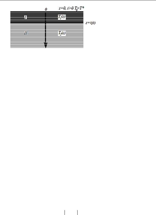
1. Statement of the problem. Let us look at a one-dimensional cooling problem followed by freezing of wet soil with the initial temperature Т0 over the freezing temperature ТФ (Т0 > ТФ) filling a flat semi-infinite space (Fig. 1).

17

Russian Journal of Building Construction and Architecture

I is the area of half-frozen soil

II is the area of thawed soil

Fig. 1. Geometric scheme of the thermal task of the motion of the interphase boundary: z (t) for 0 z

At the moment of time t = 0 on the surface z = 0 the temperature Т* is set rapidly and then maintained for all t > 0, lower than that of freezing ТФ (T* < ТФ). As a result, the frozen layer dξ, is formed whose thickness increases with time.

The law of the motion of the freezing boundary and temperature distribution in the areas of frozen and thawed soil has to be found [15—18]. In order to obtain a practical calculation method considering the combination of major factors contributing to freezing of wet soil, the following assumptions have to be made:

а) a research object (thawed and frozen soil) is modeled as being a soild body;

b)a soil material has to be homogeneous and coarse-grained structured;

c)moisture migration is considered insignificant.

Under these conditions it is necessary to solve the problem of temperature field interfacing in the moving freezing front.

In order to find the temperature field, a system of two heat conductivity equations needs to be solved where unless there are heat source for constant thermal and physical characteristics, are as follows for frozen and thawed soil respectively:

18

Here ϰ1, λ1, ϰ2, λ2 are the coefficients of temperature and heat conductivity for the frozen and thawed soil respectively; dξ / dt is the rate of motion of the interface boundary; ρ1 is the density of the frozen phase; L is the specific freezing heat.

2. Solution method and its analysis. In order to solve the equations (1) and (2) the operational Laplace transform is used [9, 10, 20] which involves search of the solution not for the time function f(t) but its image f (P). The image is generated using the transform in relation to the variable t:

where Р is a complex number (the Laplace parameter).

After finding the solution in the images, the original is determined using the inverse Laplas transform. In most cases inverse transformation can be performed using tables of standard transforms [7]. Let us use the transforms (5) for the equations (1) and (2), which is identical to multiplying their left and right sides by e−Pt followed by integration using t from 0 to ∞:

Integrating the left part step by step (6), we get:

d2T

The right part ofthe expression(6) takesthe form 1 dz21 .

Equalizing the right and left part (6) and performing identicaloperationswiththe equation(2), we get corresponding imaging equations:

They are regular linear nonhomogeneoues second-order equations with constant coefficients. Their solutions in the image spece are sums of the solutions of the general homogeneous and particular nonhomogeneous equations [22]. In case of an even initial temperature distributuion the particular solutions (7) and (8) are obvious. As

d2T2 0, dz2

19