2.2 Information theory

2.2.1 Entropy

2.40Fact (properties of entropy) Let X be a random variable which takes on n values.

(i)0 ≤ H(X) ≤ lgn.

(ii)H(X) = 0 if and only if pi = 1 for some i, and pj = 0 for all j =i (that is, there is no uncertainty of the outcome).

(iii)H(X) = lgn if and only if pi = 1/n for each i, 1 ≤ i ≤ n (that is, all outcomes are equally likely).

2.41Definition The joint entropy of X and Y is defined to be

H(X,Y ) = − P(X = x,Y = y)lg(P(X = x,Y = y)),

x,y

where the summation indices x and y range over all values of X and Y , respectively. The definition can be extended to any number of random variables.

2.42Fact If X and Y are random variables, then H(X,Y ) ≤ H(X)+H(Y ), with equality if and only if X and Y are independent.

2.43Definition If X, Y are random variables, the conditional entropy of X given Y = y is

H(X|Y = y) = − P(X = x|Y = y)lg(P(X = x|Y = y)),

x

where the summation index x ranges over all values of X. The conditional entropy of X

given Y , also called the equivocation of Y about X, is

H(X|Y ) = P(Y = y)H(X|Y = y),

y

where the summation index y ranges over all values of Y .

2.44Fact (properties of conditional entropy) Let X and Y be random variables.

(i)The quantity H(X|Y ) measures the amount of uncertainty remaining about X after Y has been observed.

(ii)H(X|Y ) ≥ 0 and H(X|X) = 0.

(iii)H(X,Y ) = H(X) + H(Y |X) = H(Y ) + H(X|Y ).

(iv)H(X|Y ) ≤ H(X), with equality if and only if X and Y are independent.

2.2.2Mutual information

2.45Definition The mutual information or transinformation of random variables X and Y is

I(X;Y ) = H(X) − H(X|Y ). Similarly, the transinformation of X and the pair Y , Z is defined to be I(X;Y,Z) = H(X) − H(X|Y,Z).

2.46Fact (properties of mutual transinformation)

(i)The quantity I(X;Y ) can be thought of as the amount of information that Y reveals about X. Similarly, the quantity I(X;Y,Z) can be thought of as the amount of information that Y and Z together reveal about X.

(ii)I(X;Y ) ≥ 0.

(iii)I(X;Y ) = 0 if and only if X and Y are independent (that is, Y contributes no information about X).

(iv)I(X;Y ) = I(Y ;X).

2.47Definition The conditional transinformation of the pair X, Y given Z is defined to be

IZ(X;Y ) = H(X|Z) − H(X|Y,Z).

2.48Fact (properties of conditional transinformation)

(i)The quantity IZ(X;Y ) can be interpreted as the amount of information that Y provides about X, given that Z has already been observed.

(ii)I(X;Y,Z) = I(X;Y ) + IY (X;Z).

(iii)IZ(X;Y ) = IZ(Y ;X).

2.3 Complexity theory

2.3.1 Basic definitions

The main goal of complexity theory is to provide mechanisms for classifying computational problems according to the resources needed to solve them. The classification should not depend on a particular computational model, but rather should measure the intrinsic difficulty of the problem. The resources measured may include time, storage space, random bits, number of processors, etc., but typically the main focus is time, and sometimes space.

2.49Definition An algorithm is a well-defined computational procedure that takes a variable input and halts with an output.

Of course, the term “well-defined computational procedure” is not mathematically precise. It can be made so by using formal computational models such as Turing machines, random-access machines, or boolean circuits. Rather than get involved with the technical intricacies of these models, it is simpler to think of an algorithm as a computer program written in some specific programming language for a specific computer that takes a variable input and halts with an output.

It is usually of interest to find the most efficient (i.e., fastest) algorithm for solving a given computational problem. The time that an algorithm takes to halt depends on the “size” of the problem instance. Also, the unit of time used should be made precise, especially when comparing the performance of two algorithms.

2.50Definition The size of the input is the total number of bits needed to represent the input in ordinary binary notation using an appropriate encoding scheme. Occasionally, the size of the input will be the number of items in the input.

2.51Example (sizes of some objects)

(i)The number of bits in the binary representation of a positive integer n is 1 + lgn bits. For simplicity, the size of n will be approximated by lgn.

(ii)If f is a polynomial of degree at most k, each coefficient being a non-negative integer at most n, then the size of f is (k + 1)lgn bits.

(iii)If A is a matrix with r rows, s columns, and with non-negative integer entries each

2.52Definition The running time of an algorithm on a particular input is the number of primitive operations or “steps” executed.

Often a step is taken to mean a bit operation. For some algorithms it will be more convenient to take step to mean something else such as a comparison, a machine instruction, a machine clock cycle, a modular multiplication, etc.

2.53Definition The worst-case running time of an algorithm is an upper bound on the running time for any input, expressed as a function of the input size.

2.54Definition The average-case running time of an algorithm is the average running time over all inputs of a fixed size, expressed as a function of the input size.

2.3.2Asymptotic notation

It is often difficult to derive the exact running time of an algorithm. In such situations one is forced to settle for approximations of the running time, and usually may only derive the asymptotic running time. That is, one studies how the running time of the algorithm increases as the size of the input increases without bound.

In what follows, the only functions considered are those which are defined on the positive integers and take on real values that are always positive from some point onwards. Let

fand g be two such functions.

2.55Definition (order notation)

(i)(asymptotic upper bound) f(n) = O(g(n)) if there exists a positive constant c and a positive integer n0 such that 0 ≤ f(n) ≤ cg(n) for all n ≥ n0.

(ii)(asymptotic lower bound) f(n) = Ω(g(n)) if there exists a positive constant c and a positive integer n0 such that 0 ≤ cg(n) ≤ f(n) for all n ≥ n0.

(iii)(asymptotic tight bound) f(n) = Θ(g(n)) if there exist positive constants c1 and c2, and a positive integer n0 such that c1g(n) ≤ f(n) ≤ c2g(n) for all n ≥ n0.

(iv)(o-notation) f(n) = o(g(n)) if for any positive constant c > 0 there exists a constant n0 > 0 such that 0 ≤ f(n) < cg(n) for all n ≥ n0.

Intuitively, f(n) = O(g(n)) means that f grows no faster asymptotically than g(n) to within a constant multiple, while f(n) = Ω(g(n)) means that f(n) grows at least as fast asymptotically as g(n) to within a constant multiple. f(n) = o(g(n)) means that g(n)is an upper bound for f(n) that is not asymptotically tight, or in other words, the function f(n) becomes insignificant relative to g(n) as n gets larger. The expression o(1) is often used to signify a function f(n) whose limit as n approaches ∞ is 0.

2.56Fact (properties of order notation) For any functions f(n), g(n), h(n), and l(n), the following are true.

(i)f(n) = O(g(n)) if and only if g(n) = Ω(f(n)).

(ii)f(n) = Θ(g(n)) if and only if f(n) = O(g(n)) and f(n) = Ω(g(n)).

(iii)If f(n) = O(h(n)) and g(n) = O(h(n)), then (f + g)(n) = O(h(n)).

(iv)If f(n) = O(h(n)) and g(n) = O(l(n)), then (f · g)(n) = O(h(n)l(n)).

(v)(reflexivity) f(n) = O(f(n)).

(vi)(transitivity) If f(n) = O(g(n)) and g(n) = O(h(n)), then f(n) = O(h(n)).

2.57Fact (approximations of some commonly occurring functions)

(i)(polynomial function) If f(n) is a polynomial of degree k with positive leading term, then f(n) = Θ(nk).

(ii)For any constant c > 0, logc n = Θ(lgn).

(iii)(Stirling’s formula) For all integers n ≥ 1,

(iv)lg(n!) = Θ(nlgn).

2.58Example (comparative growth rates of some functions) Let and c be arbitrary constants with 0 < < 1 < c. The following functions are listed in increasing order of their asymptotic growth rates:

2.3.3Complexity classes

2.59Definition A polynomial-time algorithm is an algorithm whose worst-case running time function is of the form O(nk), where n is the input size and k is a constant. Any algorithm whose running time cannot be so bounded is called an exponential-time algorithm.

Roughly speaking, polynomial-time algorithms can be equated with good or efficient algorithms, while exponential-time algorithms are considered inefficient. There are, however, some practical situations when this distinction is not appropriate. When considering polynomial-time complexity, the degree of the polynomial is significant. For example, even

60 Ch. 2 Mathematical Background

though an algorithm with a running time of O(nln ln n), n being the input size, is asymptotically slower that an algorithm with a running time of O(n100), the former algorithm may be faster in practice for smaller values of n, especially if the constants hidden by the big-O notation are smaller. Furthermore, in cryptography, average-case complexity is more important than worst-case complexity — a necessary condition for an encryption scheme to be considered secure is that the corresponding cryptanalysis problem is difficult on average (or more precisely, almost always difficult), and not just for some isolated cases.

2.60Definition A subexponential-time algorithm is an algorithm whose worst-case running time function is of the form eo(n), where n is the input size.

A subexponential-time algorithm is asymptotically faster than an algorithm whose running time is fully exponential in the input size, while it is asymptotically slower than a polynomial-time algorithm.

2.61Example (subexponential running time) Let A be an algorithm whose inputs are either elements of a finite field Fq (see §2.6), or an integer q. If the expected running time of A is

where c is a positive constant, and α is a constant satisfying 0 < α < 1, then A is a subexponential-time algorithm. Observe that for α = 0, Lq[0,c] is a polynomial in lnq, while for α = 1, Lq[1,c] is a polynomial in q, and thus fully exponential in lnq.

For simplicity, the theory of computational complexity restricts its attention to decision problems, i.e., problems which have either YES or NO as an answer. This is not too restrictive in practice, as all the computational problems that will be encountered here can be phrased as decision problems in such a way that an efficient algorithm for the decision problem yields an efficient algorithm for the computational problem, and vice versa.

2.62Definition The complexity class P is the set of all decision problems that are solvable in polynomial time.

2.63Definition The complexity class NP is the set of all decision problems for which a YES answer can be verified in polynomial time given some extra information, called a certificate.

2.64Definition The complexity class co-NP is the set of all decision problems for which a NO answer can be verified in polynomial time using an appropriate certificate.

It must be emphasized that if a decision problem is in NP, it may not be the case that the certificate of a YES answer can be easily obtained; what is asserted is that such a certificate does exist, and, if known, can be used to efficiently verify the YES answer. The same is true of the NO answers for problems in co-NP.

2.65Example (problem in NP) Consider the following decision problem:

COMPOSITES

INSTANCE: A positive integer n.

QUESTION: Is n composite? That is, are there integers a,b > 1 such that n = ab?

COMPOSITES belongs to NP because if an integer nis composite, then this fact can be verified in polynomial time if one is given a divisor a of n, where 1 < a < n(the certificate in this case consists of the divisor a). It is in fact also the case that COMPOSITES belongs to co-NP. It is still unknown whether or not COMPOSITES belongs to P.

2.66 Fact P NP and P co-NP.

The following are among the outstanding unresolved questions in the subject of complexity theory:

1.Is P = NP?

2.Is NP = co-NP?

3.Is P = NP ∩co-NP?

Most experts are of the opinion that the answer to each of the three questions is NO, although nothing along these lines has been proven.

The notion of reducibility is useful when comparing the relative difficulties of problems.

2.67Definition Let L1 and L2 be two decision problems. L1 is said to polytime reduce to L2, written L1 ≤P L2, if there is an algorithm that solves L1 which uses, as a subroutine, an algorithm for solving L2, and which runs in polynomial time if the algorithm for L2 does.

Informally, if L1 ≤P L2, then L2 is at least as difficult as L1, or, equivalently, L1 is no harder than L2.

2.68Definition Let L1 and L2 be two decision problems. If L1 ≤P L2 and L2 ≤P L1, then

L1 and L2 are said to be computationally equivalent.

2.69Fact Let L1, L2, and L3 be three decision problems.

(i)(transitivity) If L1 ≤P L2 and L2 ≤P L3, then L1 ≤P L3.

(ii)If L1 ≤P L2 and L2 P, then L1 P.

2.70Definition A decision problem L is said to be NP-complete if

(i)L NP, and

(ii)L1 ≤P L for every L1 NP.

The class of all NP-complete problems is denoted by NPC.

NP-complete problems are the hardest problems in NP in the sense that they are at least as difficult as every other problem in NP. There are thousands of problems drawn from diverse fields such as combinatorics, number theory, and logic, that are known to be NP- complete.

2.71Example (subset sum problem) The subset sum problem is the following: given a set of positive integers {a1,a2,... ,an} and a positive integer s, determine whether or not there

2.72Fact Let L1 and L2 be two decision problems.

(i)If L1 is NP-complete and L1 P, then P = NP.

(ii)If L1 NP, L2 is NP-complete, and L2 ≤P L1, then L1 is also NP-complete.

(iii)If L1 is NP-complete and L1 co-NP, then NP = co-NP.

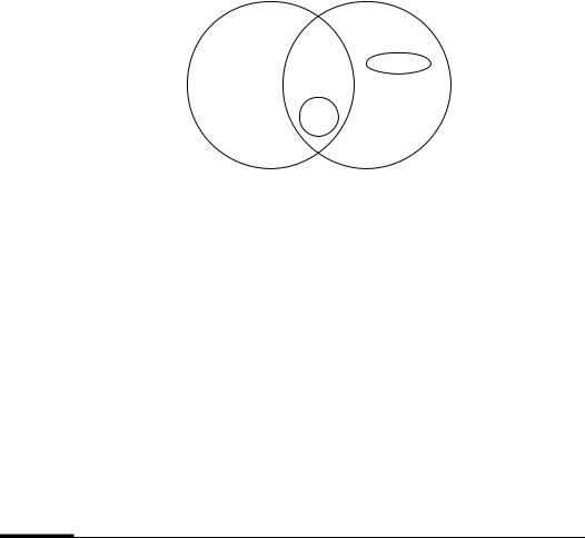
By Fact 2.72(i), if a polynomial-time algorithm is found for any single NP-complete problem, then it is the case that P = NP, a result that would be extremely surprising. Hence, a proof that a problem is NP-complete provides strong evidence for its intractability. Figure 2.2 illustrates what is widely believed to be the relationship between the complexity classes P, NP, co-NP, and NPC.

Fact 2.72(ii) suggests the following procedure for proving that a decision problem L1 is NP-complete:

Figure 2.2: Conjectured relationship between the complexity classes P, NP, co-NP, and NPC.

1.Prove that L1 NP.

2.Select a problem L2 that is known to be NP-complete.

3.Prove that L2 ≤P L1.

2.73Definition A problem is NP-hard if there exists some NP-complete problem that polytime reduces to it.

Note that the NP-hard classification is not restricted to only decision problems. Observe also that an NP-complete problem is also NP-hard.

2.74Example (NP-hard problem) Given positive integers a1,a2,... ,an and a positive integer s, the computational version of the subset sum problem would ask to actually find a

subset of the ai which sums to s, provided that such a subset exists. This problem is NP- hard.

2.3.4 Randomized algorithms

The algorithms studied so far in this section have been deterministic; such algorithms follow the same execution path (sequence of operations) each time they execute with the same input. By contrast, a randomized algorithm makes random decisions at certain points in the execution; hence their execution paths may differ each time they are invoked with the same input. The random decisions are based upon the outcome of a random number generator. Remarkably, there are many problems for which randomized algorithms are known that are more efficient, both in terms of time and space, than the best known deterministic algorithms.

Randomized algorithms for decision problems can be classified according to the probability that they return the correct answer.

2.75Definition Let A be a randomized algorithm for a decision problem L, and let I denote an arbitrary instance of L.

(i)A has 0-sided error if P(A outputs YES | I’s answer is YES ) = 1, and P(A outputs YES | I’s answer is NO ) = 0.

(ii)A has 1-sided error if P(A outputs YES | I’s answer is YES ) ≥ 12 , and P(A outputs YES | I’s answer is NO ) = 0.