

prt%3A978-0-387-35973-1%2F16
.pdfM
Machine Readable Geographic Data
Feature Catalogue
Magik, Smallworld
Smallworld Software Suite
Management of Linear
Programming Queries
MLPQ Spatial Constraint Database System
Manhattan Distance
Distance Metrics
Manifold
Spatial Data Transfer Standard (SDTS)
Manifold Rules
Smallworld Software Suite
Manifolds
Smallworld Software Suite
Mantel Test
CrimeStat: A Spatial Statistical Program for the Analysis of Crime Incidents
Map Accuracy
Spatial Data Transfer Standard (SDTS)
Map, Bi-Plot
Geographic Dynamics, Visualization And Modeling
Map, Centrographic Timeseries
Geographic Dynamics, Visualization And Modeling
Map Data
Photogrammetric Products
Map Distribution
Data Infrastructure, Spatial
Map Generalization
ANNE RUAS
Laboratory COGIT, IGN-France, Saint-MandŽ, France
Synonyms
Generalization
Definition
Map generalization is the name of the process that simpliÞes the representation of geographical data to produce a map at a certain scale with a deÞned and readable legend. To be readable at a smaller scale, some objects are removed; others are enlarged, aggregated and displaced one to another, and all objects are simpliÞed. During the process, the information is globally simpliÞed but stays readable and understandable.
The smaller the scale, the less information is given per square kilometer. Conversely, the larger the scale, the more detailed is the area mapped for the same map size. For

632 Map Overhaul
a given size of map sheet, nearly the same quantity of information is given for different scales, either privileging the density of Þeld information (for larger scale) or the spatial extension (for smaller scale).
This process is used both in manual and digital cartography.
Main Text
Generalisation can be Þrst deÞned by means of graphical constraints and scale. On a map the information is represented by means of symbols. These symbols are coded representations which ensure the interpretation of the meaning. These symbols have minimum sizes that ensure not only good perception but also the recognition of the symbols and their associated meaning. As an example, a very small black polygon representing a building will be seen as a dot and not a building. In the same way two symbols too close one to another will be seen as a single symbol even if in the real world they represent two different entities. These graphical constraints are called legibility or readability constraints. When represented on a map the graphical objects are not a faithful representation of the entitiesÕ sizes at a given scale but are symbolic representations which maximize communication of information.
In order to respect graphical constraints, some objects are enlarged and some are displaced one to another. These geometric distortions are minor at the large scale (1:2,000Ð1:10,000), common at the medium scale (1:15,000Ð1:50,000) and frequent and very large at small scales. As an example a 6 m width road represented by a line of 0.6 mm on a map is enlarged 10 times at 1:100,000 and 100 times at 1:1,000,000! Of course, when the scale decreases it is physically not possible to enlarge and displace all objects: many objects are removed, some are aggregated, and they are all simpliÞed. These operations of enlargement, displacement, selection, aggregation and geometric simpliÞcations are the main operations of generalization. There is a good large amount of literature devoted to deÞning and specifying the operators and algorithms of generalization.
But generalization can also be deÞned through a more geographical view point. A geographical representationÑbeing a map or a data baseÑrepresents the real world at a certain level of detail. This level of detail implicitly deÞnes the type of information represented and their reasonable use. Geographical phenomena have a certain size and they can only be depicted within a certain scale range. Generalization is a process that aggregates and simpliÞes the information in order to make apparent more general concepts through their representation. When scale decreases some concepts disappear while oth-
ers appear. The transition between scales can by smooth and continuous for some themes or abrupt for others. Generally networks are preserved but their density decreases, while small size objects such as houses are changed into urban areas, dots and even nothing. MŸller [2] speaks of change under scale progression (CUPS) to characterize these transformations through scale.
The complexity of the automation of the generalization process is due to the diversity of geographical information and its contextual nature. Generalization should preserve relationships and properties that are, most of the time, implicit. Current models of generalization rely on optimization techniques or on a multiagent system paradigm.
Cross References
Abstraction of GeoDatabases
Generalization and Symbolization
Recommended Reading
1.McMaster, R., ButtenÞeld, B.: Map Generalization. Longman, Harlow (1991)
2.MŸller, J-C., Lagrange, J.-P., Weibel, R.: GIS and GeneralizationÐMethodology and Practice. Taylor and Francis, London, UK (1995)
3.Mackaness, W., Ruas, A., Sarjakoski, L.T.: Generalisation of Geographic Information: Cartographic Modelling and applications. Elsevier, Burlington, MA, USA (2007)
Map Overhaul
Positional Accuracy Improvement (PAI)
Map Quality
Positional Accuracy Improvement (PAI)
Map-Matching
DIETER PFOSER
RA Computer Technology Institute, Athens, Greece
Definition
Sampling vehicular movement using GPS is affected by error sources. Given the resulting inaccuracy, the vehicle tracking data can only be related to the underlying road network by using map-matching algorithms.

MapWindow GIS |
633 |
Main Text
Tracking data is obtained by sampling movement, typically using GPS. Unfortunately, this data is not precise due to the measurement error caused by the limited GPS accuracy, and the sampling error caused by the sampling rate, i. e., not knowing where the moving object was in between position samples. A processing step is needed that matches tracking data to the road network. This technique is commonly referred to as map matching.
Most map-matching algorithms are tailored towards mapping current positions onto a vector representation of a road network. Onboard systems for vehicle navigation utilize dead reckoning besides continuous positioning to minimize the positioning error and to produce accurate vehicle positions that can be easily matched to a road map. For the purpose of processing tracking data, the entire trajectory, given as a sequence of historic position samples, needs to be mapped. The fundamental difference in these two approaches is the error associated with the data. Whereas the data in the former case is mostly affected by the measurement error, the latter case is mostly concerned with the sampling error.
Cross References
Dynamic Travel Time Maps
Floating Car Data
Recommended Reading
1.Brakatsoulas, S., Pfoser, D., Sallas, R., Wenk, C.: On mapmatching vehicle tracking data. In: Proc. 31st VLDB conference, pp. 853Ð864 (2005)
Mapping
Public Health and Spatial Modeling
Mapping and Analysis for Public Safety
Hotspot Detection, Prioritization, and Security
Maps, Animated
Geographic Dynamics, Visualization And Modeling
Maps On Internet
Web Mapping and Web Cartography
MapServ
University of Minnesota (UMN) Map Server
MapServer
Quantum GIS
Web Feature Service (WFS) and Web Map Service (WMS)
MapWindow GIS
DANIEL P. AMES, CHRISTOPHER MICHAELIS,
ALLEN ANSELMO, LAILIN CHEN, HAROLD DUNSFORD
Department of Geosciences, Idaho State University,
Pocatello, ID, USA
Synonyms |
|
|
Open-source GIS; Free GIS; Programmable GIS compo- |
|
|
M |
||
nents; .NET framework; ActiveX components |
||
Definition |
|
|
MapWindow GIS is an open source geographic informa- |
|
|
tion system that includes a desktop application and a set |
|
|
of programmable mapping and geoanalytical components. |
|
|
Because it is distributed as open source software under the |
|
|
Mozilla Public License, MapWindow GIS can be repro- |
|
|
grammed to perform different or more specialized tasks |
|
|
and can be extended as needed by end users and devel- |
|
|
opers. MapWindow GIS has been adopted by the United |
|
|
States Environmental Protection Agency as a platform for |
|
|
its BASINS watershed analysis system and is downloaded |
|
|
over 3000 times per month by end users who need a free |
|
|
GIS data viewer and programmers who need tools for com- |
|
|
mercial and non-commercial software applications. |
|
|
Main Text |
|
|
MapWindow GIS is a desktop open source GIS and set of |
|
|
programmable objects intended to be used in the Microsoft |
|
|
Windows operating system. Because it is developed using |
|
|
the Microsoft .NET Framework, it is optimized for the |
|
|
Windows environment and can be extended by program- |
|
|
mers using the Visual Basic and C# languages. The Map- |
|
|
Window GIS desktop application plug-in interface sup- |
|
|
ports custom tool development by end users and the Map- |
|
|
Window Open Source team. Additionally, software devel- |
|

634 Marginalia
opers can use the core MapWindow ActiveX and .NET programming components to add GIS mapping and geoprocessing functionality to custom standalone applications.
MapWindow GIS has been adopted by the United States Environmental Protection Agency, United Nations University and others as a development and distribution platform for several environmental models including BASINS/HSPF, FRAMES-3MRA and SWAT. Other users and developers have modiÞed and applied MapWindow GIS for use in the Þelds of transportation, agriculture, community planning and recreation. MapWindow GIS is continually maintained by an active group of nearly 50 student and volunteer developers from around the world who regularly release updates and bug Þxes through the www. MapWindow.org web site.
Cross References
Open-Source GIS Libraries
Marginalia
Metadata and Interoperability, Geospatial
Market and Infrastructure for Spatial Data
PETER KEENAN
UCD Business School, University College Dublin,
Dublin, Ireland
Synonyms
Spatial information; Geographic information
Definition
GIS combines hardware and software to allow the storage and manipulation of spatial data. GIS applications typically combine speciÞc spatial data with data on the general geographic features of an area. The availability and cost of this general data is an important factor in the more widespread adoption of spatial techniques. The spatial data market is the system enabling the transaction of business between buyers and sellers of such data. This system must reward those who collect spatial data and protect their rights over that data while making the data available to users under reasonable conditions.
Historical Background
GIS applications are comparatively resource-intensive, as they require more complex software and consequently more powerful hardware than many common applications of Information Technology (IT). However, the rapid development of IT means that sophisticated GIS software is now readily available and that the computer technology required for this software is now a small proportion of cost of using GIS. Nevertheless, while hardware and software developments have been favorable to the widespread use of GIS, the ready availability of spatial data is also a critical requirement for greater GIS use. In traditional IT applications for example, business data processing, most of the data used originates within an organization and is often the result of the use of the technology. GIS was typically Þrst employed by organizations with existing non-computerized spatial data and was used to build and manage large computerized spatial data-sets. However, as GIS use has extended to a wider user community, many potential spatial applications have a much smaller proportion of unique data collected for that speciÞc application and organization. This internal data, collected for a particular project, only becomes useful when combined with existing general geographic data sourced outside the organization. For example, information on the spatial location of retail outlets may only become useful when linked with other spatial data on shared transportation networks and demographic data for the region. Many organizations, across a wide variety of sectors, will operate in the same geographic space. These will require similar data on the general geography of the region in which they operate; this can be combined with their own spatially referenced datasets to meet their speciÞc needs. Such organizations may have little in common, other than their shared location in the same geographic region and therefore a need for spatial data about their area of operations. Consequently, applications as diverse as fuel delivery, mobile phone service provision and emergency service dispatch will have in interest in using the same spatial data.
Scientific Fundamentals
The Þrst requirement for spatial data availability is that it must be available in an appropriate format for the varied range of applications that might arise in a geographic region. While a large amount of spatial data has already been collected for developed countries, this may not be in a format suitable for the full range of possible applications for that data. In most cases traditional government mapping agencies, such as the Ordnance Survey in the UK or the Bundesamt fŸr Kartographie und GeodŠsie in Germany, now have complete digital databases of their carto-

Market and Infrastructure for Spatial Data |
635 |
graphic resources. However, the traditional focus of these agencies has been on the production of maps, rather than the use of spatial data for computer processing, and the organization of their spatial database reßects this orientation. New technologies such as remote sensing and global positioning systems (GPS) have allowed other private sector organizations collect large amounts of spatial data. Private sector spatial data providers are likely to more aware of the need to organize their data in a way which will make it useful to the maximum number of potential users. Local, regional and national public authorities will generate spatial data for the areas under their administration. However, these public organizations will collect and represent their spatial data in a way suitable for their own needs, which may not be ideal for other potential users. Therefore, much of the spatial data needed for GIS applications has already been collected, but it is not always in a format suitable for all potential users. However, the existence of spatial data is only the starting point for its widespread use. There are at least two further requirements: potential users of the data must be aware that it is available and the data must be provided at an economic cost.
While there are challenging technical issues relating to synthesis of spatial data, there are a number of initiatives to address these problems. Several countries have launched spatial data infrastructure (SDI) initiatives to provide a framework for better integrating the collection and use spatial data [1]. SDI frameworks may include spatial data clearinghouses, which can be deÞned as a computerized facility for searching, viewing, transferring, ordering, advertising, and disseminating spatial data across the Internet. In the US, the Federal Geographic Data Committee deÞnes the United States national SDI as an umbrella of policies, standards, and procedures under which organizations and technologies interact to foster more efÞcient use, management; and production of geospatial data [2]. In the US, the SDI has evolved to better integrate all forms of public data. The objective is to make this data available over the Internet and the Geospatial One-Stop (GOS) initiative (www.geo-one-stop.gov/) aims to provide a single point of access to this data. Consequently, SDI initiatives can be integrated with a geoportal which provides distributed access to the spatial data. Geoportals can primarily provide access to spatial data or can provide services which provide the result of spatial processing [3]. While it may take some time, these initiatives suggest that appropriate technical standards will emerge and that these challenges can be successfully overcome [4].
The indexation of suitable data sources can exploit the fact that spatial data has a unique location reference and can be organized with respect to this location. Consequently, an index can be produced of all data, spatial
and non-spatial, relating to a particular spatial location. A geolibrary is one approach to the organization of information in a spatially referenced structure. A geolibrary allows search for content, both spatial and non-spatial, by geographic location in addition to traditional searching methods. The concept of a geolibrary originated in the 1990s [5] and the Alexandria digital library at the University of California, Santa Barbara is generally regarded as the Þrst major prototype geolibrary (webclient.alexandria. ucsb.edu/). The geolibrary model was further deÞned within the GIS community by the Workshop on Distributed geolibraries: Spatial Information Resources, convened by the Mapping Science Committee of the US National Research Council in June 1998. Geolibraries are based on the spatial referencing of data; this data need not be either digital or spatial in nature. However, the geolibrary concept is especially useful as a means of organizing spatial data [6].
In principle, geolibraries should provide access to all types of data, both spatial and non-spatial. These resources should be centrally indexed, even if the physical storage is distributed. As more spatial data becomes available, this allows a vast number of potential combinations of these
data-sets, facilitating a wide range of applications. How- M ever, there must be a clear economic incentive for spatial
data owners to make their data available to other potential users. Spatial data may originate from organizations that see themselves as spatial data suppliers. These may be public sector bodies, with pricing policies set by government or they may be purely private sector companies seeking to proÞt from the demand for spatial data. Public policy towards spatial data pricing differs greatly across different countries. In the US, the federal government regards spatial data as a public good. Basic spatial data should logically only be collected once, in the US it is seen as appropriate for the government to do this and then make this data available at little or no cost to the public. In contrast, government policy in Canada and in most European countries is to seek to recover some or all the cost of spatial data collection from those who use it [7]. However, where data is sold by public agencies, rather than given away, there is more incentive to reorganize that data to meet the needs of potential users. While basic spatial data is free in the US, there are many private sector data providers who add value to this basic data for a fee, making it more useful for an extended range of applications.
Other spatial data-sets may originate in organizations whose primary role is not spatial data collection. Such organizations collect data primarily for their own needs, but may make it available to others if there is an incentive for doing so. For example, an electricity supply utility will have GIS data on the location of its power lines.

Mathematical Foundations of GIS |
637 |
products has become something of a de facto standard. These proprietary standards may be extended over time to include features which facilitate a spatial data market. However, if a proprietary format becomes dominant, then data provision can be greatly inßuenced by the dominant software vendor as well as the data providers, which may restrict the growth of the market. Data standards also originate in standards initiatives originating from collective organizations such as the GeoData Alliance (www.geoall. net). Such organizations work to facilitate open standards for the exchange of data. There are also initiatives to provide models relevant to the spatial data market; the Geospatial Digital Rights Management (GeoDRM) initiative of the Open Geospatial Consortium (OGC) (www. opengeospatial.org) is one example.
The spatial data market is likely to evolve to a situation where spatial software can connect electronically to spatial libraries to obtain spatial information. Data would be available in these libraries in a format containing embedded information on license restrictions. The software would allow use of this data in accordance with the license restrictions and would facilitate extension of a license as required. Digital watermarking could be included in spatial data-sets and used to trace data use. The spatial data market can evolve to take advantage of approaches developed in the e-commerce domain to encourage the sharing of spatial data, facilitating the use of spatial data in a wide range of potential applications.
Cross References
Data Infrastructure, Spatial
Information Services, Geography
OGCÕs Open Standards for Geospatial Interoperability
Recommended Reading
1.Masser, I.: The future of spatial data infrastructures. ISPRS Workshop on Service and Application of Spatial Data Infrastructure, XXXVI (4/W6). Swets & Zeitlinger B.V, Hangzhou, China (2005)
2.FGDC: Framework, Introduction and GuideBook. Federal Geographic Data Committee, Washington (1997)
3.Bernard, L., et al.: Towards an SDI Research Agenda. 11 EC-GIS Workshop. Alghero, Sardinia (2005)
4.Maguire, D.J., Longley, P.A.: The emergence of geoportals and their role in spatial data infrastructures. Comput. Environ. Urban Syst. 29(1), 3Ð14 (2005)
5.Goodchild, M.F.: The Geolibrary, Innovations in GIS V. In: Carver, S. (ed.), pp. 59Ð68. Taylor and Francis, London (1998)
6.Boxall, J.: Geolibraries, the Global Spatial Data Infrastructure and Digital Earth. Int. J. Spec. Libr. 36(1), 1Ð21 (2002)
7.Craglia, M., Masser, I.: Access to Geographic Information: a European Perspective. J. Urban Regional Inf. Syst. Assoc. (URISA) 15(APA I), 51Ð59 (2003)
8.Onsrud, H., et al.: Public Commons of Geographic Data: Research and Development Challenges. Geographic Information Science,
Third International Conference, GIScience, Adelphi, MD, USA, 2004. Springer, Heidelberg (2004)
Market-Basket Analysis
Frequent Itemset Discovery
Marketing Information System
Decision-Making Effectiveness with GIS
Markov Random Field (MRF)
Hurricane Wind Fields, Multivariate Modeling
Mash-Ups
Information Services, Geography
M
Massive Evacuations
Emergency Evacuation Plan Maintenance
Mathematical Foundations of GIS
TIMOTHY G. FEEMAN
Department of Mathematical Sciences,
Villanova University, Villanova, PA, USA
Definition
¥Geodesy is the branch of mathematics concerned with the shape and area of the earth and with the location of points on it.
¥Cartography is the art, science, and practice of making maps.
¥A map projection, or simply a projection, is any system-
atic representation of the earthÕs surface onto another surface.
¥ The Global Positioning System, or GPS, comprises a network of satellites that orbit the earth and, by radio communications with land-based receivers, enable the accurate determination of the coordinates of points on the earthÕs surface.
¥Spherical geometry is the study of lines, angles, and areas on a spherical surface.
638 Mathematical Foundations of GIS
Historical Background
The foundation of geographical information science (GIS) lies in our ability to determine the size and shape of the earth, locate points on its surface, measure its features, and to portray the earth in maps. Thus, geodesy and cartography form the basis of GIS. In turn, both of these subjects are built on strong mathematical foundations.
The Shape and Size of the Earth
In this age of space exploration, photographs of Earth and other heavenly bodies taken from space offer convincing evidence that EarthÕs basic shape is spherical. This conception of a spherical Earth has endured, though not without some lapses, at least since the sixth century B.C., when Anaximander and Thales of Miletus, two of the earliest classical Greek geometers, described the earth as a sphere positioned at the center of a huge celestial sphere to which were Þxed the other visible planets and stars.
Towards the end of the seventeenth century, Isaac NewtonÕs work on gravitation and planetary motion led him to conclude that Earth had the shape of an ellipsoid, ßattened at the poles and somewhat bulging around the equator. NewtonÕs conjecture was conÞrmed by French-spon- sored expeditions to Peru and Lapland during the 1730s in which arcs of meridians at high and low latitudes were measured. In the early 1800s, Gauss and others provided further veriÞcations. Since the introduction of satellite technology, new measurements have resulted in the development of several reference ellipsoids, including the World Geodetic Systems ellipsoid of 1984 (WGS 84, for short), developed by the US Defense Mapping Agency, and the Geodetic Reference System ellipsoid of 1980 (GRS 80), adopted by the International Union of Geodesy and Geophysics in 1979.
When the highest level of precision is needed, an ellipsoid provides the best mathematical model for the earthÕs shape. In this article, for simplicityÕs sake, a spherical Earth is assumed, with measurements and calculations made accordingly.
Assuming the earth to be a sphere, the single most important measurement is its circumference, which was estimated by Eratosthenes of Alexandria in roughly 230 B.C.
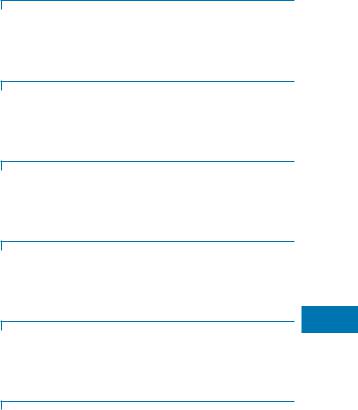
Eratosthenes knew that, at noon on any given day of the year, the angle of the sun above the horizon would be different at two different places located north and south of one another. Assuming the earth to be a sphere and all of the sunÕs rays to be parallel, Eratosthenes called upon a basic geometric fact Ð that a line transversal to two parallel lines will make equal angles with both Ð to conclude that the difference between the angles of the sun would correspond to the central angle of the portion of the
Mathematical Foundations of GIS, Figure 1 The sun is overhead at Syene (S). The angle of the sun at Alexandria (A) is the same as the central angle
earthÕs circumference between the two points (Fig. 1). He also knew that, at noon on the summer solstice, the sun shone directly overhead in the town of Syene (now Aswan, Egypt), famously illuminating a well there. Eratosthenes then determined that, on the summer solstice, the noonday sun in Alexandria was one-Þftieth part of a full circle (7.2¡) shy of being directly overhead. It followed that the distance between Syene and Alexandria must be oneÞftieth part of a full circumference of the earth. The distance between the two towns was measured to be about 5000 stadia (approximately 500 miles). Multiplication by 50 yielded EratosthenesÕ remarkably accurate estimate of 250000 stadia, about 25000 miles, for the circumference of the earth. The basic method employed by Eratosthenes is completely valid and is still used today.
In fact, the equatorial and polar radii and circumferences of the earth are different, because of the earthÕs ellipsoidal shape. The mean radius of the earth is approximately 6371 kilometers.
Scientific Fundamentals
Location
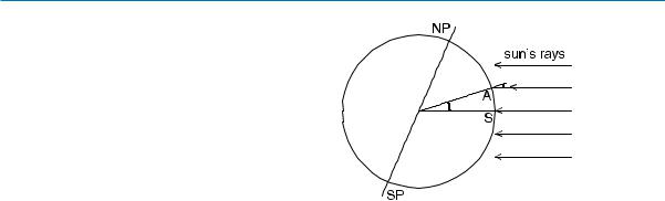
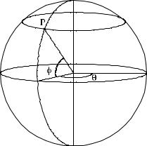
The latitude of any given point is deÞned to be the difference between the angles made by the sun at noon at the point in question and at the equator. This is illustrated in Fig. 2. Latitude is designated as north (N) or south (S) according to which hemisphere the point lies in. The points at the same latitude form a circle whose plane is parallel to that of the equator. Thus, a circle of latitude is called a parallel.
As the earth rotates about its axis, the position of the sun in the sky changes, ascending from the eastern horizon at dawn to its zenith at noon, then descending until it sets in the west. The arrival of local solar noon, the moment at which the sun reaches its zenith, is a simultaneous event at
Mathematical Foundations of GIS |
639 |
Mathematical Foundations of GIS, Figure 2 The point P has longitude θ and latitude φ
all points along a semi-circular arc, called a meridian, that extends from the north pole to the south pole. Where two meridians come together at the poles, they form an angle that is the basis for determining longitude. The difference in longitudes of two locations is the portion of a full circle through which the earth rotates between the occurrences of local solar noon at the two places. Thus, the measurement of longitude is fundamentally a problem of the measurement of time.
One way to measure time differences between two places is by the relative positions in the sky of various celestial bodies, such as certain stars, the planets, or the moons of Jupiter. The astrolabe and the sextant were among the tools developed to measure these positions, and elaborate tables were compiled showing known positions of celestial objects. Alternatively, longitude can be determined using two clocks, one set to the time at a Þxed location and the other to local time. Though sufÞciently accurate clocks are readily available today, their introduction just a few centuries ago marked a giant leap in the technology of navigation. The Þrst sea-worthy chronometer was developed in England by John Harrison and presented to the English Longitude Board in 1735, though it took some years of reÞnements in size, weight, and ease of reproduction for the new clocks to catch on.
In addition to the technical problem of measuring time differences, there is the political issue of deciding which meridian will serve as the reference, or prime meridian, for longitude calculations. Ptolemy placed his prime meridian through the Canary Islands. Others have used the meridians through Mecca, Jerusalem, Paris, Rome, Copenhagen, the Cape Verde Islands, St. Petersburg, Philadelphia, and more. After 1767, when the Royal Observatory in Greenwich, England, published the most comprehensive tables
of lunar positions available, sailors increasingly calculated |
|
||||||
their longitude from Greenwich. This practice became ofÞ- |
|
||||||
cial in 1884 when the International Meridian Conference |
|
||||||
established the prime meridian at Greenwich. Longitude is |
|
||||||
designated as east (E) or west (W) according to whether |
|
||||||
local noon occurs before or after local noon in Greenwich. |
|
||||||
Latitude and longitude together give a complete system for |
|
||||||
locating points on the earthÕs surface. |
|
||||||
Coordinates |
|
||||||
Where cartographers often measure angles in degrees, here |
|
||||||
angles will be measured in radians in order to simpli- |
|
||||||
fy trigonometric computations. Also, positive and nega- |
|
||||||
tive angle measurements will be used instead of the direc- |
|
||||||
tional designations north/south or east/west, with south |
|
||||||
and west assigned negative values. The symbols θ and ϕ |
|
||||||
will denote longitude and latitude, respectively. Thus, the |
|
||||||
point with longitude 75¡ W and latitude 40¡ N has coor- |
|
||||||
dinates (θ = −75π/180, φ = 40π/180) while the point |
|
||||||
with longitude 75¡ E and latitude 40¡ S has coordinates |
|
||||||
(θ = 75π/180, φ = −40π/180). |
|
||||||
For the Cartesian coordinate system in three-dimension- |
|
||||||
al space, the line through the north and south poles will |
|
||||||
M |
|||||||
be taken as the z-axis, with the north pole on the pos- |
|||||||
itive branch. The plane of the equator corresponds to |
|
||||||
the xy-plane with the positive x-axis meeting the equa- |
|
||||||
tor at the prime meridian and the positive y-axis meeting |
|
||||||
the equator at the point with longitude π/2 (or 90¡ E). |
|
||||||
On a sphere of radius R, then, the point with longi- |
|
||||||
tude |
θ |
and latitude ϕ will have Cartesian coordinates |
|
||||
(x, y, z) |
= (R cos(θ ) cos(φ), R sin(θ ) cos(φ), R sin(φ)). |
|
|||||
Conversely, latitude and longitude can be recovered from |
|
||||||
the Cartesian coordinates. The equation φ = arcsin(z/R) |
|
||||||
determines φ uniquely as an angle between −π/2 and π/2. |
|
||||||
Also, θ |
satisÞes the equations tan(θ ) = y/x, cos(θ ) = |
|
|||||
x/ |
x2 + y2 |
, and sin(θ ) = y/ |
x2 + y2 |
. Any two of these |
|
||
together will determine a unique angle θ between −π and π .
Distance
The distance between two points is the length of the shortest path connecting the two points. On a sphere, the path must lie entirely on the surface and, so, cannot be a straight line segment as it is in a plane. Instead, the shortest path is the straightest possible one which, intuitively, is an arc of the largest possible circle, called a great circle.
A great circle on a sphere is the intersection of the sphere with a plane that contains the center of the sphere. Every great circle has a radius equal to that of the sphere. The equator is a great circle while each meridian is half of a great circle. Any two great circles must intersect each
640 Mathematical Foundations of GIS
other at a pair of antipodal points. Indeed, the planes deÞned by the circles will intersect in a line through the sphereÕs center, which, therefore, will intersect the sphere at two opposite points.
Any two non-antipodal points on the sphere determine a unique great circle, namely the intersection of the sphere with the plane generated by the two points together with the center of the sphere. The two points divide this circle into two arcs, the shorter of which is the shortest path connecting the points. If O denotes the center of a sphere of radius R and by A and B the two points of interest, then the distance between A and B along the shorter great circle arc is equal to the product of R and the central angle, measured
OA and OB. (This is |
|
in radians, formed by the two vectors −→ |
−→ |
essentially the deÞnition of radian measure.)
To derive a formula for distance in terms of the longitudes and latitudes of the points in question, assume for simplicityÕs sake that the sphere has radius R = 1 unit and let the points A and B have longitudes θ1 and θ2 and latitudes φ1 and φ2, respectively. Converting to three-dimensional Cartesian coordinates,
A= (cos φ1 cos θ1, cos φ1 sin θ1, sin φ1) and
B= (cos φ2 cos θ2, cos φ2 sin θ2, sin φ2) .
From vector geometry, the cosine of the angle between the
−→ −→
two vectors OA and OB is given by their dot product divided by the product of the vectorsÕ lengths, each of which is 1 in this case. The value of the dot product is
−→ −→
OA • OB
=cos φ1 cos θ1 cos φ2 cos θ2 + cos φ1 sin θ1 cos φ2 sin θ2
+sin φ1 sin φ2
=cos φ1 cos φ2 (cos θ1 cos θ2 + sin θ1 sin θ2)
+sin φ1 sin φ2
=cos φ1 cos φ2 cos(θ1 − θ2) + sin φ1 sin φ2 .
The angle between the vectors is then
−→ −→ angle = arccos(OA • OB)
= arccos(cos φ1 cos φ2 cos(θ1 − θ2) |
(1) |
|
|
+ sin φ1 sin φ2) . |
|
Now multiply this angle by the radius of the sphere to get the distance. That is,
distance = R arccos(cos φ1 cos φ2 cos(θ1 − θ2)
(2)
+ sin φ1 sin φ2) .
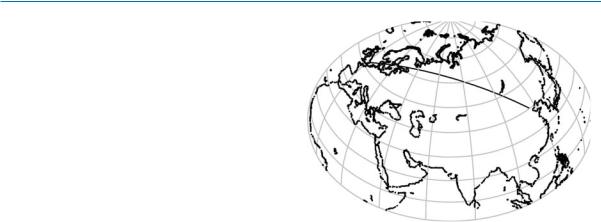
For example, London, England, has longitude θ1 = 0 and latitude φ1 = 51.5π/180, while θ2 = 116.35π/180 and
Mathematical Foundations of GIS, Figure 3 Great circle route from London to Beijing
φ2 = 2π/9 are the coordinates of Beijing. Therefore, the central angle between London and Beijing is about 1.275 radians. The mean radius of the earth is about R = 6371 kilometers and, hence, the great circle distance from London to Beijing is approximately 1.275R, or 8123 kilometers. The great circle route is illustrated in Fig. 3.
The most important map projection for the depiction of great circle routes is the gnomonic projection, which is constructed by projecting a spherical globe onto a plane tangent to the globe using a light source located at the globeÕs center. Any two points on the sphere, along with the light source for the projection, deÞne a plane that intersects the sphere in a great circle and the plane of the map in a straight line, which is, therefore, the image of the great circle joining the points. In other words, the gnomonic projection has the property that the shortest route connecting any two points A and B on the sphere is projected onto the shortest route connecting their images on the ßat map.
The gnomonic projection was most likely known to Thales of Miletus and would have been particularly useful to navigators and traders of the Golden Age of Greece, a time of intensiÞed trade and geographical discovery during which the Bronze Age gave over to the Age of Iron.
The gnomonic projection can be constructed from elementary geometry. Place a globe of radius R on a ßat piece of paper with the south pole at the bottom and with a projecting light source at the center of the globe. Points on or above the equator wonÕt project onto the paper, so the map will show only the southern hemisphere. Arrange the mapÕs coordinate axes so that the prime meridian is projected onto the positive x-axis, in which case the image of the meridian at longitude θ makes an angle of θ , measured counter-clockwise, with the positive x-axis. The parallels, meanwhile, will be shown on the map as concentric circles having the pole as their common center. When the globe is