

Joye M.Cryptographic hardware and embedded systems.2005
.pdf6J. Waddle and D. Wagner
between the grouping and the power consumption in the traces, so, for 
 and
and 
Given these traces as inputs, the algorithms try to decide whether the groupings (and hence the guess for the key) are correct by distinguishing these distributions.
3.2The Generic DPA Subroutine
Both algorithms use a subroutine DPA after their preprocessing step. For our purposes, this subroutine simply takes the two groups of traces,  and
and  a threshold value
  and determines whether the groups’ totalled traces differ by more than
  at any sample time. If the difference of the totalled traces is greater than
  at any point, DPA returns 1, indicating that
  and
and  have different distributions; if the difference is no more than
  at any point, DPA returns 0, indicating that it thinks
  and
and  are identically distributed.
When using the DPA subroutine, it is most important to pick the threshold,  appropriately. Typically, to minimize the impact of false positives and false negatives,
  should be half the difference. This is perhaps unexpected since false positives are actually far more likely than false negatives when using a
midpoint threshold test since |
false positives can occur if any of the |
times’ |
|
samples sum deviates above |
while false negatives require exactly the correlated |
||
time’s samples to deviate below |
The reason for not choosing to equalize the |
||
probabilities is that false negatives are far more detrimental than false positives: an attack suggesting two likely subkeys is more helpful than an attack suggesting none.
An equally important consideration in using DPA is whether  is large enough compared to the noise to reduce the probability of error. Typically, the samples’ noise components will be independent and the summed samples’ noise will be Gaussian, so we can can achieve negligible probability of error by using
  large enough that
  is some constant multiple of the standard deviation.
DPA runs in time  Each run of DPA decides the correctness of only one guessed grouping, however, so an attack that tries
  groupings runs in time
TEAM LinG
Towards Efficient Second-Order Power Analysis |
7 |
4Our Second-Order Attacks
The two second-order variants of DPA that we discuss are Zero-Offset 2DPA and FFT 2DPA. The former is applied in the special but not necessarily unlikely situation when the power correlation times for the two bits are coincident (i.e., the random bit  and the masked bit
  are correlated with the power consumption at the same time). The latter attack applies to the more general situation where the attacker does not know the times of correlation; it discovers the correlation with only slight computational overhead but pays a price in the number of required samples.
4.1Zero-Offset 2DPA
Zero-Offset 2DPA is a very simple variation of ordinary first-order DPA that can be applied against systems that employ masking in such a way that both the random bit  and the masked intermediate bit
  correlate with the power consumption at the same time. In the language of our model,
The coincident effect of the two masked values may seem to be too specialized of a circumstance to occur in practice, but it does come up. The motivation for this attack is the claim by Coron and Goubin [3] that some techniques suggested by Messerges [4] were insecure due to some register containing the multi-bit intermediate value  or its complement
  Since Messerges assumes a power consumption model based on Hamming weight, it was not clear how a first-order attack would exploit this register. However, we observe that such a system can be attacked (even in the Hamming model) by a Zero-Offset 2DPA that uses as its intermediate value the exclusive-or of the first two bits of
  Another example of a situation with coincident power consumption correlation is in a paired circuit design that computes with both the random and masked inputs in parallel.
Combining  with Equation (3), we see that in a correct grouping:
In an incorrect grouping, |
is distributed exactly as in the general uncorre- |
|
lated case in Equation (4). |
|
|
Note that in a correct grouping, when |
the influence of the two bits |
|
cancel, leaving |
while when |
the influences of the two |
bits combine constructively and we get |
In the former |
|
case, there appears to be no influence of the bits on the power consumption distribution, but in the latter case, the bits contribute a bimodal component. The bimodal component has mean 0, however, so it would not be apparent in a first-order averaging analysis.
Zero-offset 2DPA exploits the bimodal component for the  case by simply squaring the samples in the power traces before running straight DPA.
TEAM LinG

8J. Waddle and D. Wagner
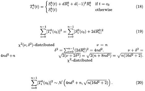
Why does this work? Suppose we have a correct grouping and consider the expected values for the sum of the squares of the samples at time  in the two groups:
 if
if 
if 
The above derivations use the fact that if |
then |
(i.e., |
||
has |
distribution with |
degree of freedom and non-centrality parameter |
||
|
and the expected value of a |
random variable is |
|
|
|
Thus, the expected difference of the |
sum of products for the |
samples |
|
is |
while the expected difference for incorrect groupings is clearly 0. In |
|||
Section A.1, we show that the difference of the groups’ sums of products is essentially Gaussian with standard deviation
For an attack that uses a DPA threshold value at least  standard deviations from the mean, we will need at least
  traces. This
  blowup factor may be substantial; recall that
  is in units of the standard deviation of the noise, so it may be significantly less than 1.
The preprocessing in Zero-Offset-DPA takes time  After this preprocessing, each of
  subsequent guessed groupings can be tested using DPA in
TEAM LinG
Towards Efficient Second-Order Power Analysis |
9 |
time  for a total runtime of
  It is important to keep in mind when comparing these run times that the number
  of required traces for Zero-Offset-DPA can be somewhat larger than would be necessary for first-order DPA—if a first-order attack were possible.
A Natural Variation: Known-Offset 2DPA. If the difference  is non-zero but known, a similar attack may be mounted. Instead of calculating the squares of the samples, the adversary can calculate the lagged product:
where the addition |
is intended to be cyclic in |
|
This lagged product |
at the correct offset |
has properties similar |
to the squared samples discussed above, and can be used in the same way.
4.2FFT 2DPA
Fast Fourier Transform (FFT) 2DPA is useful in that it is more general than Zero-Offset 2DPA: it does not require that the times of correlation be coincident, and it does not require any particular information about  and
and 
To achieve this, it uses the FFT to compute the correlation of a trace with itself—an autocorrelation. The autocorrelation  of a trace
  is also defined on values
  but this argument is considered an offset or lag value rather than an absolute time. Specifically, for
  and
and
The argument |
in |
is understood to be cyclic in |
so |
||
that |
and we really only need to consider |
|
|||
To see why |
might be useful, recall Equation (3) and notice that most |
||||
of the terms of |
are of the form |
in fact, the only terms |
|||
that differ are where or |
is |
or |
This observation suggests a way to |
||
view the sum for |
by splitting it up by the different types of terms from |
||||
Equation (3), and in fact it is instructive to do so. To simplify notation, |
let |
||||
|
|
the set of “interesting” indices, where the terms of |
|||
are “unusual” when |
Assuming |
|
|
||
TEAM LinG

10 J. Waddle and D. Wagner
and we can distribute and recombine terms to get
Using Equation (12) and the fact that  when X and Y are independent random variables, it is straightforward to verify that
  when
when  its terms in that case are products involving some 0-mean independent random variable (this is exactly what we show in Equation (15)). On the other hand,
  involves terms that are products of dependent random variables, as can be seen by reference to Equation (10). We make frequent use of Equation (12) in our derivations in this section and in Appendix A.2.
This technique requires a subroutine to compute the autocorrelation of a trace:
The  in line 3 is the squared
  of the complex number
  (i.e.,
 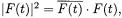 where
where  denotes the complex conjugate of
The subroutine FFT computes the usual Discrete Fourier Transform:
and Inv-FFT computes the Inverse Discrete Fourier Transform:
In the above equations,  is a complex primitive mth root of unity (i.e.,
  and
and  for all
The subroutines FFT,Inv-FFT, and therefore Autocorrelate itself all run in time 
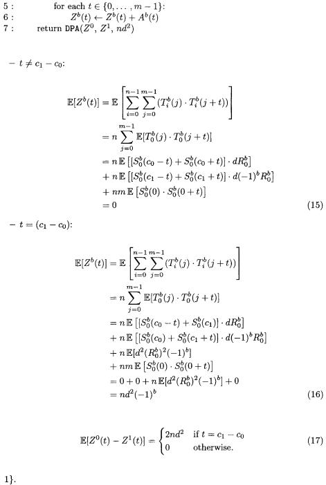
We can now define the top-level FFT-2DPA algorithm:
TEAM LinG
Towards Efficient Second-Order Power Analysis |
11 |
What makes this work? Assuming a correct grouping, the expected sums are:
So in a correct grouping, we have
In incorrect groupings, however,  for all
In Section A.2, we see that this distribution is closely approximated by a Gaussian with standard deviation 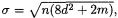 so that an attacker who
TEAM LinG
12 J. Waddle and D. Wagner
wishes to use a threshold at least  standard deviations away from the mean
needs  to be at least about
Note that the noise from the other samples contributes significantly to the standard deviation at  so this attack would only be practical for relatively short traces and a significant correlated bit influence (i.e., when
  is
is
small and |
is not much smaller than 1). |
|
The preprocessing in FFT-2DPA runs in time |
After this pre- |
|
processing, |
however, each of guessed groupings |
can be tested using DPA in |
time |
for a total runtime of |
amortizing to |
if |
Again, when considering this runtime, it is important to keep |
|
in mind that the number of required traces can be substantially |
larger than |
would be necessary for first-order DPA—if a first-order attack were |
possible. |
FFT and Known-Offset 2DPA. It might be very helpful in practice to use the FFT in second-order power analysis attacks for attempting to determine the offset of correlation. With a few traces, it could be possible to use an FFT to find the offset  of repeated computations, such as when the same function is computed with the random bit
  at time
  and with the masked bit
  at time
With even a few values of  suggested by an FFT on these traces, a KnownOffset 2DPA attack could be attempted, which could require far fewer traces than straight FFT 2DPA since Known-Offset 2DPA suffers from less noise amplification.
5Conclusion
We explored two second-order attacks that attempt to defeat masking while minimizing computation resource requirements in terms of space and time.
The first, Zero-Offset 2DPA, works in the special situation where the masking bit and the masked bit are coincidentally correlated with the power consumption, either canceling out or contributing a bimodal component. It runs with almost no noticeable overhead over standard DPA, but the number of required power traces increases more quickly with the relative noise present in the power consumption.
The second technique, FFT 2DPA, works in the more general situation where the attacker knows very little about the device being analyzed and suffers only logarithmic overhead in terms of runtime. On the other hand, it also requires many more power traces as the relative noise increases.
In summary, we expect that Zero-Offset 2DPA and Known-Offset 2DPA can be of some practical use, but FFT 2DPA probably suffers from too much noise amplification to be generally effective. However, if the traces are fairly short and the correlated bit influence fairly large, it can be effective.
TEAM LinG
Towards Efficient Second-Order Power Analysis |
13 |
References
l.Paul Kocher, Joshua Jaffe, and Benjamin Jun, “Differential Power Analysis,” in proceedings of Advances in Cryptology—CRYPTO ’99, Springer-Verlag, 1999, pp. 388-397.
2.Thomas Messerges, “Using Second-Order Power Analysis to Attack DPA Resistant
Software,” Lecture Notes in Computer Science, 1965:238-??, 2001.
3.Jean-Sébastien Coron and Louis Goubin, “On Boolean and Arithmetic Masking against Differential Power Analysis”, in Proceedings of Workshop on Cryptographic Hardware and Embedded Systems, Springer-Verlag, August 2000.
4.Thomas S. Messerges, “Securing the AES Finalists Against Power Analysis Attacks,” in Proceedings of Workshop on Cryptographic Hardware and Embedded Systems, Springer-Verlag, August 1999, pp. 144-157.
ANoise Amplification
In this section, we attempt to characterize the distribution of the estimators that we use to distinguish the target distributions. In particular, we show that the estimators have near-Gaussian distributions and we calculate their standard deviations.
A.1 Zero-Offset 2DPA
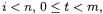
As in Section 4.1, we assume that the times of correlation are coincident, so that  From this, we get that the distribution of the samples in a correct grouping follows Equation (5):
The sum
is then a |
random variable with |
degrees of freedom |
|
and non-centrality parameter |
|
|
It has mean |
and standard deviation |
|
|
|
A common rule of thumb is that |
random variables with over |
||
thirty degrees of freedom are closely approximated by Gaussians. We expect  so we say
TEAM LinG

14 J. Waddle and D. Wagner
Similarly, we obtain  which, since
  we approximate with
The difference of the summed squares is then
A.2 FFT 2DPA
Recalling our discussion from Section 4.2, we want to examine the distribution of
when |
Its standard deviation should |
dominate that of |
for |
|
(for simplicity, we assume |
|
|
In Section 4.2, we saw that |
We would now like to |
||
calculate its |
standard deviation. |
|
|
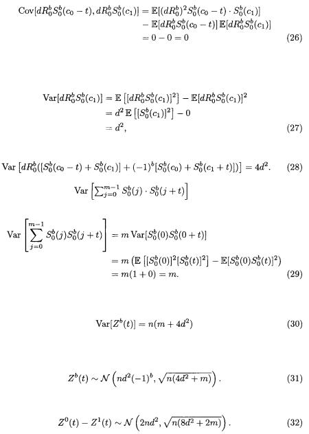
In the following, we liberally use the fact that |
|
|
|
where Cov[X, Y] is the covariance of X and Y  We would often like to add variances of random variables that are not independent; Equation (24) says we can do so if the random variables have 0 covariance.
Since the traces are independent and identically distributed,
where we were able to split the variance in the last line since the two terms have 0 covariance.
TEAM LinG
Towards Efficient Second-Order Power Analysis |
15 |
To calculate  note that its terms have 0 covariance. For example:
since the expectation of a product involving an independent 0-mean random variable is 0. Furthermore, it is easy to check that each term has the same variance, and
for a total contribution of
The calculation of |
is similar since its terms also |
have covariance 0 and they all have the same variance. Thus,
Finally, plugging Equations (28) and (29) into Equation (25), we get the result
and the corresponding standard deviation is  As in Section A.1, we expect
  to be large and we say
Finally, we get the distribution of the difference:
TEAM LinG