

Eure K.W.Adaptive predictive feedback techniques for vibration control
.pdfβ(z) = β 0 + β 1 z −1 + β 2 z −2 + +β p z − p
δ(z) = δ 0 + δ 1 z −1 + δ 2 z −2 + +δ p z − p
Disturbances which consist of only a single-input periodic signal may be represented by the finite-difference model shown in Eq. (4.22)41.
d( k ) = η1d( k − 1) + η2d( k − 2 )+ +ηnd d( k − nd ) |
(4.22) |
In Eq.(4.22), nd is the disturbance model order and is twice the number of commensurable frequencies in the disturbance signal. Taking the z transform of Eq.(4.22), results in Eq. (4.23).
η( z )d( z ) = 0
where
η( z ) = 1 − η1 z −1 − η2 z −2 − −ηnd z −nd
Premultiplying Eq. (4.21) byη( z ) and using Eq. (4.23) results in
η( z )α( z )y( z ) = η( z )β( z )u( z )
which may be written as
~~
α(z)y(z) = β(z)u(z)
where
~ |
|
~ |
−1 |
~ |
−2 ~ |
|
− p−nd |
α ( z ) = η( z )α( z ) = I m |
− α 1 z |
|
− α 2 z |
− −α p z |
|
||
~ |
~ |
~ |
−1 |
~ |
~ |
− p−nd |
|
β |
( z ) = η( z )β( z ) = β0 |
− β1 z |
− β2 z |
−2 − −β p z |
|||
(4.23)
(4.24)
In Eq. (4.24) the system order is p + nd rather than p. This is due to the fact that the model given by Eq. (4.24) has imbedded within the parameters an exact model of the disturbance41. The value of nd is twice the number of periodic disturbances acting on the system. The resulting system model provides an exact input output map for the discretetime system being identified given that the periodic disturbance is the only disturbance acting on the system. A similar proof for MIMO systems with periodic disturbances may be found in Ref. [41] were it is proven that an exact input-output map may be obtained for MIMO systems in the presence of periodic disturbances.
49
4.7 Experimental Results
The GPC algorithm with feedforward and a noise predictor was implemented on a Texas Instrument C-30 chip. The plant to be regulated is shown in Fig. 3.1. The accelerometer signal was measured by the B&K analyzer as shown in Fig 3.2. The control input enters the plant through the piezo mounted on the bottom center of the aluminum plate. The plant output to be regulated is the accelerometer signal taken at the top center of the aluminum plate. A block diagram of the plant and control system is shown in Fig. 3.2. The disturbance d is band limited to 1KHz and enters the plant at point 2 of Fig. 3.2. The plant output is the accelerometer signal taken at point 3. The control input is applied to the plant at point 1 of Fig. 3.2. Low pass filters and amplifiers were used where appropriate. The controller has a sample rate of 2.5 KHz and has input signals of y, the filtered and amplified accelerometer signal and d, the disturbance measurement. The controller outputs u, the control signal. The total reduction presented for some of the plots is give to demonstrate the overall performance of the controller. This value is obtain by integrating the spectrum of the openand closed-loop accelerometer autospectrum. The closed-loop integrated spectrum is then divided by the open-loop integrated spectrum. The result is then expressed in dB. The total reductions presented throughout this thesis are obtained in this manner.
Since the implementation in this study is not adaptive, we must first estimate an ARMAX model of the plant in order to design a controller. This is accomplished by applying two independent white noise signals (band limited to 1Kz), to point 2 of Fig. 3.2 and at u. With both these random inputs applied, the system output y of Fig. 3.2 is measured. The two input data vectors and the one output vector are then used to approximate an ARMAX model of the system. It is important to note that the ARMAX model represents both the plexiglass box and the filters and amplifiers used in the controller loop. The form of the model is that of Eq. (4.1). The ARMAX model was then used to find the GPC controller coefficients shown in Eq. (4.9).
50

-10 |
|
|
|
|
|
|
|
|
-20 |
|
|
|
|
|
|
|
|
-30 |
|
|
|
|
|
|
|
|
-40 |
|
|
|
|
|
|
|
|
dB |
|
|
|
|
|
|
|
|
-50 |
|
|
|
|
|
|
|
|
-60 |
|
|
|
|
|
|
|
|
-70 |
|
|
|
|
|
|
|
|
-80 |
200 |
400 |
600 |
800 |
1000 |
1200 |
1400 |
1600 |
0 |
||||||||
|
|
|
Frequency, H z |
|
|
|
||
Figure 4.2 GPC Performance with Feedback/Feedforward Control
Figure 4.2 shows the autospectrum of plant output (accelerometer signal, y) without control (gray line), feedback only (dotted line), and with feedback/feedforward control (solid line). A 12th order system model was used with a sample rate of 2.5 KHz. Both control and prediction horizons were set to 12. Since the disturbance applied to the plant was band-limited white noise, no AR model could be used to predict future disturbances before they enter the plant. Therefore the second to last term in Eq. (4.9) was dropped. It is also of interest to consider the controller performance around 800 Hz. Here we see that the feedback controller is performing better than the feedback/feedforward controller. This is probably due to the fact that the feedforward path is introducing additional noise into the system around this frequency which is not created by the disturbance. This additional noise comes from leveling the output spectrum. It is a small sacrifice made in order to regulate the modal responses of the plant. It must be kept in mind that both feedback and feedback/feedforward control only penalize the amplitude squared of the sensor signal as described by the cost function. This does not guarantee that the controllers will regulate across the entire bandwidth. It does, however, mean that the overall level of the plant output will be reduced for all stable control designs.
51

-20 |
|
|
|
|
|
|
|
|
-30 |
|
|
|
|
|
|
|
|
-40 |
|
|
|
|
|
|
|
|
dB |
|
|
|
|
|
|
|
|
-50 |
|
|
|
|
|
|
|
|
-60 |
|
|
|
|
|
|
|
|
-70 |
|
|
|
|
|
|
|
|
-80 |
200 |
400 |
600 |
800 |
1000 |
1200 |
1400 |
1600 |
0 |
||||||||
|
|
|
|
Frequency, H z |
|
|
|
|
Figure 4.3 Feedback/Feedforward Tone Rejection Using Internal Noise Model
In Fig. 4.3, the plots are the autospectrum of the plant output without control (gray line), and with feedback/feedforward control plus a 2nd order internal noise model (solid line). The total reduction was 9.67 dB. A 12th order system model was used, 2nd order AR tone model, and the sample rate was 2.5 KHz. The internal noise model was formed based on a 2nd order AR model obtained by performing a system ID on the disturbance signal. The resulting AR model and the past disturbance measurements were then used to predict the future disturbance values and incorporate the last term of Eq. (4.9). Figure 4.3 shows the advantage gained by including the second to last term of Eq. (4.9) when possible. In this case, both band-limited white noise and a 800 Hz sine wave disturbance were applied to the plant through the speaker. Only the sine wave was used in the feedforward path. As seen in Fig. 4.3, this greatly attenuated the accelerometer signal due to the sine wave disturbance.
52
-20 |
|
|
|
|
|
|
|
|
-25 |
|
|
|
|
|
|
|
|
-30 |
|
|
|
|
|
|
|
|
-35 |
|
|
|
|
|
|
|
|
-40 |
|
|
|
|
|
|
|
|
dB |
|
|
|
|
|
|
|
|
-45 |
|
|
|
|
|
|
|
|
-50 |
|
|
|
|
|
|
|
|
-55 |
|
|
|
|
|
|
|
|
-60 |
|
|
|
|
|
|
|
|
-65 |
|
|
|
|
|
|
|
|
-70 |
500 |
1000 |
1500 |
2000 |
2500 |
3000 |
3500 |
4000 |
0 |
Frequency, Hz
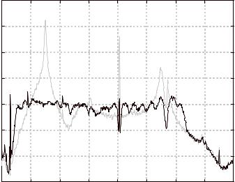
Figure 4.4 Plot of Control Using Internal Noise Model
Figure 4.4 is the autospectrum of the plant output without control (gray line), feedback (dotted line, 5.15 dB reduction), feedback with internal noise model (dashed line, 6.51 dB reduction), and feedback/feedforward control (solid line, 14.40 dB reduction). The system order was 38 and the sample rate was 10 KHz. Figure 4.4 shows broadband results using the GPC controller. Here band-limited white noise was applied as the disturbance so no AR disturbance model exists to enhance performance. The black line is the autospectrum of the accelerometer signal when the feedback/feedforward controller of Eq. (4.9) was used without the second to last term. It is of interest to compare the result obtained using feedback only, (dotted line), with that of feedback using an internal noise model, (dashed line). In both cases no feedforward was used. The system ID was performed with the disturbance on for the dashed line. For the dotted line, the system ID was done with the disturbance off. By having the disturbance on while gathering input and output data for the system ID, the resulting ID will incorporate some information about how the disturbance propagates through the plant and to the
53
accelerometer. The controller design will use this information to increase regulation as can be seen in when comparing the dashed line to the dotted line in Fig. 4.4.
The figures shown thus far used controllers with broadband internal noise models. Incorporating disturbance information into the feedback controller can be used to improve the regulation of periodic disturbances as well. For this case, a large increase in regulation may be obtained by performing the system ID in the presence of the disturbance. By doing this, an internal model of the disturbance is incorporated into the observer Markov parameters returned by the system ID41 as shown in Fig. 4.5.
1 |
|
|
|
|
|
1 |
|
|
|
|
0.8 |
|
|
|
|
|
0.8 |
|
|
|
|
0.6 |
|
|
|
|
|
0.6 |
|
|
|
|
0.4 |
|
|
|
|
|
0.4 |
|
|
|
|
0.2 |
|
|
|
|
|
0.2 |
|
|
|
|
0 |
|
|
|
|
|
0 |
|
|
|
|
-0.2 |
|
|
|
|
|
-0.2 |
|
|
|
|
-0.4 |
|
|
|
|
|
-0.4 |
|
|
|
|
-0.6 |
|
|
|
|
|
-0.6 |
|
|
|
|
-0.8 |
|
|
|
|
|
-0.8 |
|
|
|
|
-1 |
|
|
|
|
|
-1 |
|
|
|
|
-1 |
-0.5 |
0 |
0.5 |
1 |
1.5 |
-1 |
-0.5 |
0 |
0.5 |
1 |
|
|
Z plane |
|
|
|
|
|
Z plane |
|
|
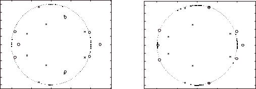
Figure 4.5 Pole-Zero Plot of OMP Without (left) & With (right) Disturbance
Figure 4.5 shows the pole zero plots of OMP obtained with disturbance off (left), and disturbance on (right). A 10th order system model and 1 KHz sampling rate were used. The disturbance was a 200 Hz sine wave. Figure 4.5 illustrates the internal disturbance model obtained by performing the system ID with the disturbance on. The figure is a polezero plot of the transfer function which describes the dynamics between the control input and accelerometer output. Both plots represent the same system (same system Markov parameters), however, the right plot contains the disturbance model. In this case, the disturbance was a 200 Hz sine wave. The plant has a mode at 300 Hz and was modeled as a 10th order system. Note the pole zero cancellation in the right plot. This plot has the same system Markov parameters as the left plot, but has different OMP41,6.
54
|
60 |
|
|
|
|
|
|
|
|
|
50 |
|
|
|
|
|
|
|
|
|
40 |
|
|
|
|
|
|
|
|
|
30 |
|
|
|
|
|
|
|
|
|
20 |
|
|
|
|
|
|
|
|
dB |
10 |
|
|
|
|
|
|
|
|
|
|
|
|
|
|
|
|
|
|
|
0 |
|
|
|
|
|
|
|
|
|
-10 |
|
|
|
|
|
|
|
|
|
-20 |
|
|
|
|
|
|
|
|
|
-30 |
|
|
|
|
|
|
|
|
|
-40 |
50 |
100 |
150 |
200 |
250 |
300 |
350 |
400 |
|
0 |
Frequency, Hz
Figure 4.6 Cancellation of Tone With Feedback Only
Figure 4.6 shows the ability of a feedback controller with an internal noise model to cancel a sine wave disturbance. Here, the autospectrum of the plant output without control (gray line), feedback only (dotted line), and feedback with internal noise model (solid line), is shown. A 20th order system model was used with a sample rate of 1 KHz. The disturbance in Fig. 4.6 was a 300 Hz tone. Since this is a resonant frequency of the plant, regulation may be performed with little control effort. The advantage of using the internal noise model may be seen by comparing the dotted line to the solid black line. Fig. 4.6 illustrates the ability of feedback control to greatly attenuate a periodic disturbance without the need of a reference source as in feedforward control.
Multiple sine waves may also be modeled in the observer Markov parameters (OMP), returned by the system ID. Figure 4.7 illustrates the performance of a broadband controller which was designed using the OMP containing the disturbance model.
55

10 |
|
|
|
|
|
|
|
|
0 |
|
|
|
|
|
|
|
|
-10 |
|
|
|
|
|
|
|
|
-20 |
|
|
|
|
|
|
|
|
-30 |
|
|
|
|
|
|
|
|
dB |
|
|
|
|
|
|
|
|
-40 |
|
|
|
|
|
|
|
|
-50 |
|
|
|
|
|
|
|
|
-60 |
|
|
|
|
|
|
|
|
-70 |
|
|
|
|
|
|
|
|
-80 |
200 |
400 |
600 |
800 |
1000 |
1200 |
1400 |
1600 |
0 |
Frequency, Hz
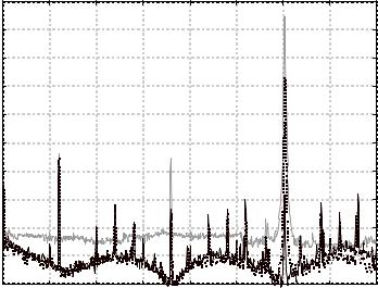
Figure 4.7 Plot of Resonance Tone Rejection
Figure 4.7 shows the autospectrum of the plant output without control (gray line), feedback (dotted line), and feedback with internal noise model (solid line). A 50th order system model was used with a sample rate of 2.5 KHz. The disturbance signal entering the plant of Fig. 4.7 was the sum of a 300 Hz sine wave, a 1100 Hz sine wave and band limited white noise. When the system ID was performed with the disturbance on, the resulting OPM contained a model of both sine wave disturbances. As can be seen by comparing the solid line to the dotted line in Fig. 4.7, the internal noise model greatly improved regulation at the frequencies of both sine wave disturbances.
The periodic disturbances in both Fig. 4.6 and 4.7 were at resonant frequencies of the plant. If the disturbance is at an off resonant frequency, regulation may still be performed if the control actuator has sufficient authority. This may be seen in Fig. 4.8.
56
0 |
|
|
|
|
|
|
|
|
-10 |
|
|
|
|
|
|
|
|
-20 |
|
|
|
|
|
|
|
|
-30 |
|
|
|
|
|
|
|
|
dB |
|
|
|
|
|
|
|
|
-40 |
|
|
|
|
|
|
|
|
-50 |
|
|
|
|
|
|
|
|
-60 |
|
|
|
|
|
|
|
|
-70 |
200 |
400 |
600 |
800 |
1000 |
1200 |
1400 |
1600 |
0 |
Frequency, Hz
Figure 4.8 Plot of Off Resonance Tone Rejection
Figure 4.8 shows the autospectrum of the plant output without control (gray line), and feedback with internal noise model (solid line). A 50th order system model was used with a sample rate of 2.5 KHz. The disturbance in Fig 4.8 was a 800 Hz tone plus band limited white noise. As can be seen in the figure, resonance response control is obtained along with cancellation of the off resonance tone. The frequency range shown in Fig. 4.8 goes up to 1.6 KHz. The spectrum analyzer in this experiment obtained the accelerometer signal after passing through the amplifiers and low pass filter as shown in Fig. 3.2. Since this is a continuous-time signal, the fact that the DSP system is running at 2.5 KHz is not related to the bandwidth shown in Fig. 4.8. The bandwidth of Fig. 4.8 is half the sample rate of the B&K analyzer, not half the DSP sample rate.
57

50 |
|
|
|
|
|
|
|
|
40 |
|
|
|
|
|
|
|
|
30 |
|
|
|
|
|
|
|
|
20 |
|
|
|
|
|
|
|
|
10 |
|
|
|
|
|
|
|
|
dB |
|
|
|
|
|
|
|
|
0 |
|
|
|
|
|
|
|
|
-10 |
|
|
|
|
|
|
|
|
-20 |
|
|
|
|
|
|
|
|
-30 |
200 |
400 |
600 |
800 |
1000 |
1200 |
1400 |
1600 |
0 |
Frequency, Hz
Figure 4.9 GPC with Internal Noise Model vs. Feedback/Feedforward
Figure 4.9 shows the autospectrum of the plant output without control (gray line), feedback with internal noise model (dotted line), and feedback/feedforward control (solid line). A 50th order system model was used for all cases with a sample rate of 2.5 KHz.
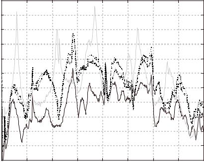
The disturbance was white noise band-limited to 1 KHz. The reason for the resonant response beyond 1 KHz is due to the fact that the filter used to band-limit the disturbance signal was a four-pole butterworth filter with a 3 dB cut-off of 1 KHz. This filter allowed enough noise beyond 1 KHz into the plant to excite the first and second resonance beyond 1 KHz. Alaising occurred due to the spectrum beyond 1.25 KHz shown in Fig. 4.9, but this is a small amount and is tolerable. Both prediction and control horizons were set to the system order. The control weighting was 0.001. Figure 4.9 compares the performance of the GPC feedback controller with an internal disturbance model to feedback/feedforward GPC control. As can be seen in the figure, the feedback/feedforward controller gave an additional 3 or 4 dB reduction around the first mode in comparison to the feedback controller.
58