Eure K.W.Adaptive predictive feedback techniques for vibration control

6.4.1 Non-Adaptive MIMO Control

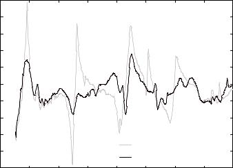
Shown in Figs. 6.4-6.7 are the accelerometer signals to be regulated by the fourchannel controller. For all figures, the gray line is the open-loop autospectrum of the acceleration in dB and the black line is the closed-loop acceleration in dB. The channel numbers correspond to the points shown in Fig. 6.3. The controller used in this case was a non-adaptive controller determined from a 75th order system identification. The system identification technique used was the batch least squares method based on the information matrix8 as described in Eq. (6.4). In order to perform the system identification, 5000 samples of input data and 5000 samples of output data for each of the four channels were used. The input data was four independent white noise sources band limited to 800 Hz. The output data was the four accelerometer signals low pass filtered at 800 Hz. The GPC11 was used to determine the controller parameters based on the OMP returned from the system identification. In the GPC algorithm, both the prediction and control horizons were set to 75 which is the order of the finite-difference model (ARX model). A control penalty of 0.0004 was used and the sampling rate was 2.5 KHz. The plots shown in Figs. 6.4-6.7 were obtained with a B&K analyzer positioned as shown in Fig. 3.2. Fifty averages were used to determine the autospectrum of the accelerometer signals. A Hanning window was applied to the data with an overlap of 50%.

89

Frequency, Hz

Figure 6.4 Plate Acceleration at Point #1 in dB

Frequency, Hz

Figure 6.5 Plate Acceleration at Point #2 in dB

90

Frequency, Hz

Figure 6.6 Plate Acceleration at Point #3 in dB

Frequency, Hz

Figure 6.7 Plate Acceleration at Point #4 in dB

Table 6.3 summarizes the results presented in Figs. 6.4-6.7.

91

Table 6.3 Total Reductions, 4 Channel Non-adaptive Controller

Total Reduction in Accelerometer Energy

dB

12.24

11.97

9.23

11.87

In Figs. 6.4-6.7 the resonant peaks in the open-loop spectrum correspond to the natural frequencies of vibration of the plate. As can be seen in these figures, the predictive feedback controller regulates the modal response of the plate. The fundamental plate mode is around 90 Hz. It was found that this mode was difficult to regulate for two reasons. The first and most important is the problem of accurately modeling the plate at this low frequency. Because the sampling rate was set to 2.5 KHz and the finitedifference order to 75, the ID at 90 Hz is difficult to determine6. The second reason for reduced performance at 90 Hz is due to the fact that the piezo has a frequency dependent response. At low frequencies, the piezo looses actuation authority.

It is also of interest to examine the radiated sound power of the non-adaptive four channel controller and compare openand closed-loop results. This is shown in Fig. 6.8- 6.9.

92

Plot of Vibration Energy

Figure 6.8 Plot of Vibration Energy

Figure 6.8 shows the plate vibration energy. The gray line is without control and the black line is with control. The total reduction in vibration energy is 7.67 dB. Figure 6.8 was obtained by scanning the plate with a laser and recording the velocity of 64 equally spaced points on the plate. Each of the 64 areas of the plate was treated as an independent vibrating mass. The total vibration energy at a fixed frequency i is given by summing the contribution from each patch for a given frequency46.

velocities for each point at frequency ωi . M is a diagonal mass matrix and the super-script

H is the Hermitian (conjugate transpose).

93

Plot of Radiated Sound Power

Figure 6.9 Plot of Radiated Sound Power

Figure 6.9 is a plot of the radiated sound power. The gray line is without control and the black line is with control. Total reduction in radiated sound power is 5.79 dB. Figure 6.9 was obtained using Eq. (6.12)46.

Here, W(ωi) is the power radiated at frequency i, ρ is the density of the medium, S is the area of the elemental radiator, ki = ωi/c where c is the speed of sound in the medium, and rhj is the distance from element h to element j. Equation (6.12) may be used to compute the radiated sound power at a given frequency i. N is the total number of elemental areas and the off-diagonal terms are due to the interactions of the individual radiators. Equation (6.12) was solved with i = 1,2,3, 800 and N = 64 to produce Fig. (6.9).

94

6.4.2 Adaptive Feedback Control

The controller performance plots shown thus far were for the non-adaptive case. The GPC control scheme may also be used in an adaptive controller to regulate plate vibrations. Equation (6.10) was applied to regulate the vibrations of the plate shown in Fig. 6.3. The results are shown in Figs. 6.10-6.13. In these figures, the four-channel block adaptive controller adapted to the conditional updating threshold, and then stopped adapting. The algorithm used blocks of 4000 data points from each of the four input and output channels. The bandwidth to be regulated was from 0 to 800 Hz and a sampling rate of 2.5 KHz was used. The control penalty was 0.0002. For all channels, the finitedifference order was 50, and the control and prediction horizons were also set to 50. The accelerometer outputs and control inputs were filtered by four pole low-pass filters set to 800 Hz. The plots shown in Figs. 6.10-6.13 are the autospectrum of the accelerometer signals obtained with a B&K analyzer. The B&K analyzer performed 50 averages and used a Hanning window with 50% overlap. The system update period was 115.73 seconds. Once every 115.73 seconds, a new block of 4000 points from each input and output was uploaded to a Pentium 166 MHz PC and used to update the control parameters if the data was found to contain a level of correlation which exceeded the set threshold. The adaptation threshold is determined by summing the elements of the matrix as described in Section 6.2. Several runs were made and a set value was determined by trial and error. The threshold value was set low enough to allow the OMP to be updated if sufficient information exist in the current block of input and output data. The threshold value must also be set high enough to prevent the OMP from drifting off if the current blocks of data do not contain sufficient information. The gray lines are open-loop and the black lines are closed-loop.

95

Frequency, Hz

Figure 6.10 Plate Acceleration at Point #1 in dB

Frequency, Hz

Figure 6.11 Plate Acceleration at Point #2 in dB

96

Frequency, Hz

Figure 6.12 Plate Acceleration at Point #3 in dB

Frequency, Hz

Figure 6.13 Plate Acceleration at Point #4 in dB

As can be seen in Figs. 6.10-6.13, the adaptive feedback controller performed slightly better than the non-adaptive controller. This occurred because in the adaptive case, the

97

controller was allowed to fine tune itself to the system to be regulated2. This is to say that the OMP are adjusted to yield the maximum level of regulation for the given system model order, horizons, and control penalty. The plant to be regulated in this case is timeinvariant. The total reductions are summarized in Table 6.4.

Table 6.4 Total Reductions, 4 Channel Adaptive Controller

Total Reduction in Accelerometer Energy

dB

14.85

15.22

10.77

13.08

The figures shown thus far present the autospectrum of the openand closed-loop accelerometer signals. However, the controller performance may also be demonstrated by plotting the magnitude of the Bode plot16 of the closed-loop system. Here, the input of the system is the disturbance input and the output is the accelerometer signal. Figures 6.14- 6.17 show the magnitude of the Bode plot for the four channel adaptive controller presented earlier. In these figures, the gray line is open-loop and the black line is closedloop.

98