
1
Diffusion MR Imaging
1.1 Introduction
1.1.1 Diffusion
Focus Point
•Particles suspended in a fluid (liquid or gas) are forced to move in a random motion called “Brownian motion.”
•Diffusion is “Brownian motion.”
Diffusion refers to the random, microscopic movement of particles due to thermal collisions. Particles suspended in a fluid (liquid or gas) are forced to move in a random motion, which is often called “Brownian motion” or pedesis (from Greek: πήδησις [meaning “leaping”]) resulting from their collision with the atoms or molecules in the gas or liquid.
This diffuse motion was named after Robert Brown, the famous English botanist, who observed under a microscope that pollen grains in water were in a constant state of agitation. It was as early as 1827 and, unfortunately, he was never able to fully explain the mechanisms that caused this motion. He initially assumed that he was observing something “alive,” but later he realized that something else was the cause of this motion since he had detected the same fluctuations when studying dead matter such as dust.
Atoms and molecules had long been theorized as the constituents of matter, and many decades later (in 1905) Albert Einstein published a paper explaining in precise detail how the motion that Brown had observed was a result of the pollen being moved by individual water molecules (Einstein, 1905). In the introduction of his paper, it is stated that
... according to the molecular-kinetic theory of heat, bodies of a microscopically visible size suspended in liquids must, as a result of thermal molecular motions, perform motions of such magnitudes that they can be easily observed with a microscope. It is possible that the motions to be discussed here are identical with so-called Brownian molecular motion; however, the data available to me on the latter are so imprecise that I could not form a judgment on the question ....
To get a feeling of the physical meaning of diffusion, consider a diffusing particle that is subjected to a variety of collisions that we can consider random, in the sense that each such event is virtually unrelated to its previous event. It makes no difference whether the particle is a molecule of perfume diffusing in air, a solute molecule in a solution, or a water molecule inside a medium diffusing due to the medium’s thermal energy.
1

2 |
Advanced MR Neuroimaging: From Theory to Clinical Practice |
Einstein described the mathematics behind Brownian motion and presented it as a way to indirectly confirm the existence of atoms and molecules in the formulation of a diffusion equation, in which the diffusion coefficient is related to the mean squared displacement of a Brownian particle.
In other words, Einstein sought to determine how far a Brownian particle travels in a given time interval.
For this purpose, he introduced the “displacement distribution,” which quantifies the fraction of particles that will traverse a certain distance within a particular timeframe, or equivalently, the likelihood that a single given particle will undergo that displacement.
Using this concept, Einstein was able to derive an explicit relationship between displacement and diffusion time in the following equation:
x2 = 6Dt |
(1.1) |
|
where x2 is the mean-squared displacement of particles during a diffusion time t, and D is the diffusion coefficient. The distribution of squared displacements takes a Gaussian form, with the peak being at zero displacement and with equal probability of displacing a given distance from the origin no matter in which direction it is measured. Actually, the Gaussian diffusion can be calculated in one, two, or three dimensions. The form of the Gaussian in one dimension is the familiar bell-shaped curve and the displacement is 2Dt. In two dimensions, if the medium is isotropic, the cross-section of the curve is circular, with the radius given by 4Dt, centered on the origin. When extended to three dimensions, the iso-probability surface is a sphere, of radius 6Dt as in Equation 1.1, and again centered on the origin.
The concept of diffusion can be easily demonstrated by adding a few drops of ink to a glass of water. The only pre-requirement is for the water in the glass to be still. Initially, the ink will be concentrated in a very small volume, and then with time, it will diffuse into the rest of the water until the concentration of the ink is uniform throughout the glass. The speed of this process of diffusion, or the rate of change of concentration of the ink, gives a measure of the property of medium where diffusion takes place. In that sense, if we could follow the diffusion of water molecules into the brain, we would reveal aspects of functionality of the normal brain tissue itself. More importantly, by understanding in more detail normal brain functionality, we would then be able to analyze the kind of changes that may occur in the brain when it is affected by various disease processes.
In other words, diffusion properties represent the microscopic motion of water molecules of the tissue; hence it can be used to probe local microstructure. As water molecules are agitated by thermal energy, they diffuse inside the body, hindered by the boundaries of the surrounding tissues or other biological barriers. By probing this movement, the reconstruction of the boundaries that hinder this motion can be visualized.
1.1.2 Diffusion in Magnetic Resonance Imaging
Magnetic resonance imaging (MRI) with its excellent soft tissue visualization and variety of imaging sequences has evolved to one of the most important noninvasive diagnostic tools for the detection and evaluation of the treatment response of cerebral tumors. Nevertheless, conventional MRI presents limitations regarding certain tumor properties, such as infiltration and grading (Hakyemez et al., 2010). It is evident that a more accurate detection of infiltrating cells beyond the tumoral margin and a more precise tumor grading would strongly enhance the efficiency of differential diagnosis. Diffusion-weighted imaging (DWI) provides

Diffusion MR Imaging |
3 |
noninvasively significant structural information at a cellular level, highlighting aspects of the underlying brain pathophysiology.
In theory, DWI is based on the freedom of motion of water molecules, which can reflect tissue microstructure; hence the possibility to characterize tumoral and peritumoral microarchitecture, based on water diffusion findings, may provide clinicians a whole new perspective on improving the management of brain tumors. Although, initially, DWI was established as an important method in the assessment of stroke (Schellinger et al., 2001), a large number of studies have been conducted in order to assess whether the quantitative information derived by DWI may aid differential diagnosis and tumor grading (Fan et al., 2006; Lam et al., 2002; Kono et al., 2001; Yamasaki et al., 2005), especially in cases of ambiguous cerebral neoplasms (Nagar et al., 2008). Moreover, DWI may also have a significant role in therapeutic follow-up and prognosis establishment in various brain lesions. Given its important clinical role, DWI should be an integral part of diagnostic brain imaging protocols (Schmainda, 2012; Zakaria et al., 2014).
1.2 Diffusion Imaging: Basic Principles
1.2.1 Diffusion-Weighted Imaging
Focus Point
•Particles suspended in a fluid (liquid or gas) are forced to move in a random motion, which is often called “Brownian motion.”
•Diffusion is considered the result of the random motion of water molecules.
•Molecular diffusion in tissues is not free, but reflects interactions with many obstacles, such as macromolecules, fibers, membranes, etc.
•By understanding normal brain diffusion, we would be able to analyze the kind of changes that may occur in the brain when it is affected by various disease processes.
•DWI represents the microscopic motion of water molecules hence probes local tissue microstructure.
As already explained, diffusion is considered the result of the random walk of water molecules inside a medium due to their thermal energy, and is described by the “Brownian” law by a diffusion constant D. Water makes up 60%–80% of human body weight. For pure water at ~37°C, D is approximately 3.4 × 10⁻³ mm2/s (Gillard et al., 2005). In an isotropic medium, diffusion is equally distributed towards all directions, described previously as the drop of ink in a glass of water. Nevertheless, it is evident that within an anisotropic medium such as human tissue, water motion will be restricted. Therefore, inside an even more complex environment, such as the human brain, cell membranes, neuronal axons, and other macromolecules act as biological barriers to free water motion, hence water mobility is considered anisotropic. In other words, in the brain, water molecules bounce, cross, and interact with tissue components. Therefore, in the presence of those obstacles, the actual diffusion distance is reduced compared to free water, and the displacement distribution is no longer Gaussian. Strictly speaking, while over very short times, diffusion reflects the local intrinsic viscosity, at longer diffusion times the effects of the obstacles become predominant. Although the observation of this displacement distribution is made on a statistical basis, it provides unique clues about the structural features and geometric organization of neural tissues on a microscopic scale, as well as changes in those features with physiological or pathological states (Le Bihan et al., 2006).
4 |
Advanced MR Neuroimaging: From Theory to Clinical Practice |
More specifically, the highly organized white-matter bundles, due to their myelin sheaths, force water to move along their axes, rather than perpendicular to them, as an apt analogy of a bundle of cables as seen in Figure 1.1.
Hence, MR can be used to probe the structural environment providing a unique opportunity to visually quantify the diffusional characteristics of tissue. This is of paramount importance in the environment of a biological sample in which the size of the area under study is so small that conventional imaging techniques are insufficient. Try to keep in mind that in 50 ms (this is considered a “typical” time interval for diffusion measurements) the diffusion distance of “free” water molecules at 37°C, will be about 17 μm. DWI is an advanced MR technique, which is based on the aforementioned Brownian motion of molecules to acquire images. One must not forget, however, that the overall signal observed in a “diffusion” MR image volume element (voxel), at a millimetric resolution, results from the integration, on a statistical basis, of all the microscopic displacement distributions of the water molecules present in this voxel. With most current MRI systems, especially those developed for human applications, the voxel size remains quite large (that is, a few mm3). The averaging and smoothing effect resulting from this scaling presumes some homogeneity in the voxel and makes it difficult to obtain a direct physical interpretation from the global parameter, unless some assumptions can be made (Le Bihan et al., 1986, 2006). The exact relationship between the diffusion properties and specific tissue microscopic features is currently the object of intensive research (Kaden et al., 2016).
Let us try and see how diffusion affects the MR signal and how this can be measured and evaluated in clinical practice.
When a patient is inserted into the homogeneous magnetic field of an MR scanner, the nuclear spins are lined up along the direction of the static magnetic field. Nevertheless, there is no such thing as a perfectly homogeneous magnetic field because it simply can’t be produced.
H2O moves harder
H2O moves easier |
|
(a) |
(b) |
FIGURE 1.1 Freeze-fractured section through a bundle of myelinated nerve fibers (a) and the apt analogy of a bundle of cables (b). It is evident that water molecules will move more easily along the direction of the nerve fibers, rather than perpendicular to them.
Diffusion MR Imaging |
5 |
Even if it could, the insertion of the patient’s susceptibility effects (such as the sinuses or bone, etc.) would make it inhomogeneous.
The effect of these external field inhomogeneities on the self-diffusion of molecules was first reported by Erwin Hahn (Hahn, 1950) who observed that: “... nuclear signals due to precessing nuclear moments contained in liquid molecules are not only attenuated by the influence of T1 and T2, but also suffer a decay due to the self-diffusion of the molecules into differing local fields established by external field inhomogeneities.”
At the same time, Bloch (Bloch, 1950) realized that the effects of diffusion can be magnified by purposely imposing a field inhomogeneity in a controlled manner. In that sense, if a radiofrequency pulse is applied, the protons will spin at different rates depending on the strength, duration, and direction of the so-called “gradient.” By applying an equal and opposite gradient, the protons will be refocused, hence information about how much the nuclear spins have moved (diffused) during this time can be acquired. In other words, stationary protons will provide a null signal after this counter-process while mobile protons, which have changed position between the two gradients, will present a signal loss.
Moving forward, in DW MRI, we simply measure the dephasing of proton spins in the presence of a gradient field (i.e., a magnetic field that spatially varies). Hence, the basic phenomenon studied is the change of a proton’s phases along the axis of the applied gradient field, which is expected to increase with “diffusion time.” The longer and stronger the gradient pulses, the more direction changes of the molecules and hence the bigger the loss of coherence and signal attenuation because of the macroscopic motion. By comparing the signal amplitude with and without the diffusion-encoding gradient applied, the portion of dephasing resulting from incoherent motion during the application of the gradient can be isolated (Jones et al., 2013).
A schematic of this sequence is presented in Figure 1.2.
It should be clear now that the brightness of each voxel of a diffusion image corresponds to the DW intensity, which in turn corresponds to the amount of diffusion weighting or gradient.
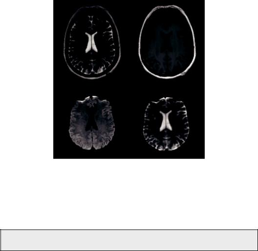
Hence, tissues closer to water (e.g., CSF) that have mobile protons, would give lower intensity while more static or solid tissues (e.g., white matter) would give a stronger signal. In that sense, DW contrast behaves like T1 weighting, or more precisely, like inverse T2 weighting. Figure 1.3 depicts an axial T2 image (a), with the corresponding T1 image (b), DW image (c), and ADC image (d), collected from a male subject.
1.2.2 The b-Value
The aforementioned signal loss would be dependent on the degree of diffusion weighting, which is referred to as the b-value. The b-value is a factor that reflects the strength and duration of the gradient pulses used to generate DW images. Therefore, to put it as simply as possible, ignoring the stationary protons and measuring the signal of the mobile protons, the amount of diffusion that has occurred in a specific direction can be determined. The b-value is described by the following mathematical equation:
b = (γGδ) |
2 |
|
− |
δ |
(1.2) |
|
|
|
|||
|
|
|
|
3 |
|
A more detailed explanation of the b-factor is obviously out of the “clinical” scope of this book, but this expression can be used to obtain an estimate of the diffusion “sensitization” for a given experiment. In this equation, is the temporal separation of the gradient pulses, δ is their duration, G is the gradient amplitude, and γ is the gyromagnetic ratio of protons (= 42.58 MHz/T) (Stejskal and Tanner, 1965). The diffusion time is assigned as (Δ – δ/3), where the second term in the expression accounts for the finite duration of the pulsed field gradients. The units
6 |
Advanced MR Neuroimaging: From Theory to Clinical Practice |
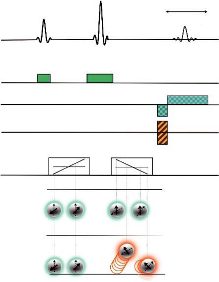
180°
Echo
90°
RF
Gsel
Gread
Gph-enc.
First diffusion gradient |
Second diffusion gradient |
Gdiff
Stationary protons
Diffusing protons
Positions after movement
FIGURE 1.2 A pulse-gradient spin-echo sequence for diffusion imaging. The standard spin-echo sequence is diffusion sensitized using a gradient pulse pair (Gdiff) so that the spin phase-shift depends on location along the first gradient pulse. The 180° radiofrequency (RF) pulse and the second gradient pulse will rephrase the static spins while diffusing spins will be “caught” out of phase.
for the b-value are s/mm–2, and the range of values typically used in clinical diffusion weighting is 800–1500 s/mm–2. The formula for the b-factor implies that we can increase diffusion weighting (DW), or “sensitization,” by increasing either gradient timing, δ or Δ, or gradient strength, G. Note that the equation for the b-value does not take into account the rising and falling edges of the diffusion gradients (see Figure 1.2) and assumes perfect rectangles. This is not actually the case, but we will discuss that in the next chapter.
Diffusion MR Imaging |
7 |
(a) |
(b) |
(c) |
(d) |
FIGURE 1.3 Axial T2 Image (a), T1 Image (b), DW image (c), and ADC image (d) collected from a male subject.
It can be shown that for a fixed diffusion weighting, the signal in a DW experiment is given by the following equation:
S = S0e |
−TE |
or S = S0e−bADC |
(1.3) |
T 2e−bD |
|
So inevitably, at this point, the question arises: What is the optimal b-value for clinical DWI?
It has been shown that for typical imaging experiments, the optimal b-value is about 1257 s/mm–2 (Jones et al., 1999). However, most studies are limited to DW imaging using b-factors of 0 and 1000. An upper b-factor around 1000 s/mm–2 has been available for most clinical scanners until now and DW imaging using these standard values has been shown to be effective in detecting and delineating restricted diffusion, for example, in acute ischemic lesions of the brain. Nevertheless, it may be more important to consider that in a clinical setting, it is advisable to maintain the same b-value for all examinations, making it easier to learn to interpret these images and become aware of the appearance of findings in various disease processes.
However, in more recent studies, it has been proposed that high b-value diffusion MR imaging can provide enhanced contrast toward different cellular components when compared to 1000 s/mm2. It is argued that the parallel analysis of low and high b-value diffusion images may provide a more comprehensive tissue characterization, enabling improved sensitivity and specificity of DW MRI to healthy tissue microstructure and subtle pathology, especially in white matter (Assaf and Basser, 2005; Ben-Amitay et al., 2012; Seo et al., 2008).
Unfortunately, such analyses may suffer from poor signal to noise ratio, leading to longer acquisition times and therefore more motion artifacts, limiting their clinical application. For more details please refer to Chapter 2.
8 |
Advanced MR Neuroimaging: From Theory to Clinical Practice |
1.2.3 Apparent Diffusion Coefficient
In Equation 1.3, S0 is the signal intensity in the absence of any T2 or diffusion weighting, TE is the echo time and D is the apparent diffusivity, usually called the Apparent Diffusion Coefficient (ADC). The term “apparent” reveals that, because tissues have a complicated structure, it is often an average measure of a number of multiple incoherent motion processes and does not necessarily reflect the magnitude of intrinsic self-diffusivity of water (Le Bihan et al., 1986; Tanner, 1978).
Hence, to reflect the fact that we are not talking about the intrinsic self-diffusivity of water, and to clarify that this estimated diffusivity comes from a sum of different spins, we use the term ADC. Please note that ADC is a calculated value based on diffusion images using at least two different b-values as shown by the following equation:
|
|
1 |
|
|
|
− |
|
DW image |
(1.4) |
||
ADC image = |
ln |
|
|||
|
|
b |
T 2w image |
|
|
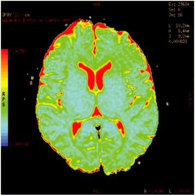
For a more accurate value of ADC, instead of two, a range of b-values can be applied and a “leastsquares” fit can be performed. ADC can also be displayed as a colored map as seen in Figure 1.4.
Going back to the b-value, the first exponential term in Equation 1.2 is the weighting due to transverse (T2) relaxation and the second term shows that diffusion induces an exponential attenuation to the signal (Price, 2007). As the diffusing spins are moving inside the field gradient, each spin is affected differently by the field, thus the alignment of the spins with each other is altered. Since the measured signal is a summation of tiny signals from all individual spins, the
FIGURE 1.4 Typical ADC parametric color map of a healthy volunteer.
Diffusion MR Imaging |
9 |
misalignment, or “dephasing,” caused by the gradient pulses results in a drop in signal intensity; the longer the diffusion distance, the more dephasing, the lower the signal (Moritani et al., 2009). The goal of DWI is to estimate the magnitude of diffusion within each voxel, i.e., the tissue microstructure, and this can be measured by the term ADC. The aforementioned parametric map of ADC values is obtained in order to facilitate qualitative measurements. The intensity of each image pixel on the ADC map reflects the strength of diffusion in the pixel. Therefore, a low value of ADC (dark signal or “cold” color) indicates restricted water movement, whereas a high value (bright signal or “warm” color) of ADC represents free diffusion in the sampled tissue (Debnam and Schellingerhout, 2011). A “quick” way to remember DWI and ADC is depicted in Figure 1.5.
A high ADC value implies high motion (free diffusion) and therefore low signal in a DW image. For example, as seen in Figure 1.3, in cerebral regions where water diffuses freely, such as CSF inside the ventricles, there is a drop in signal on the acquired DW images, whereas in areas that contain many more cellular structures and constituents (gray matter or white matter), water motion is relatively restricted and the signal on DW images is increased. Consequently, regions of CSF will present higher ADC values than other brain tissues on the parametric maps. ADC is measured in units of mm2s–1. An indicative value of ADC for pure water at room temperature is approximately
2.2 × 10⁻³ mm2s–1. Typical normal and pathological tissue ADC values are given in Table 1.1.
Free diffusion |
Restricted diffusion |
DWI |
ADC |
DWI |
ADC |
|
(a) |
|
(b) |
FIGURE 1.5 Signal intensities of DWI and ADC relative to diffusion characteristics. When diffusion is not restricted, the DWI signal is low and ADC signal is high (a). When there is restriction in diffusion the DWI signal is high and ADC is low (b).
TABLE 1.1 ADC Values (× 10−3 mm2/s) in the Normal Brain and Indicative
Disorders
ROI |
ADC value (× 10−3mm2/s) |
|
Normal Brain |
|
|
White matter |
0.84 ± 0.11 |
|
Corpus callosum |
0.75 |
± 0.15 |
CSF |
3.40 |
± 0.45 |
Thalamus |
0.83 |
± 0.14 |
Pons |
0.84 ± 0.15 |
|
Cerebellar parenchyma |
0.83 |
± 0.17 |
Disorder |
|
|
Acute infarct (cytotoxic edema) |
0.32 |
± 0.09 |
Vasogenic edema |
1.68 |
± 0.27 |
Glioblastoma multiforme |
1.27 |
± 0.46 |
Brain metastasis |
1.17 |
± 0.52 |
|
|
|

10 |
Advanced MR Neuroimaging: From Theory to Clinical Practice |
1.2.4 Isotropic or Anisotropic Diffusion?
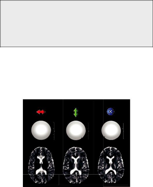
At this point it is important to clarify the concept of isotropy or anisotropy. Isotropy is derived from the Greek word isos (ἴσος, meaning “equal”) and tropos (τρόπος, meaning “way”) thus meaning “equal way” or uniform in all orientations. On the contrary, exceptions, or inequalities in Greek, are frequently indicated by the prefix “an” (meaning “the opposite of”), hence the term “anisotropy.” In that sense, anisotropy is used to describe situations where properties vary systematically, dependent on direction. An attempt to visualize a completely isotropic and gradually anisotropic voxel is depicted in Figure 1.6.
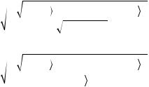
In pure water, molecules are equally likely to move in any direction, therefore, water’s diffusion properties should be isotropic. This would mean that the MR signal will be absolutely the same, irrespective of the physical direction of the applied gradients. Indeed, this is the case as shown in Figure 1.7, where three different DW images of a water phantom are depicted, one for each of the principal axes of the scanner, X, Y, and Z. But in many biological tissues, diffusion is restricted to certain directions because of the cell membranes and other organelles, for example, in directional structures such as the nerve fibers, where diffusion is preferential along the fibers rather than across them (Figure 1.1).
Areas of the brain with similar diffusion properties in every direction are said to be isotropic and independent of the direction of application of the diffusion gradients; they will have the same signal characteristics on DW images. On the other hand, anisotropic areas are characterized by different diffusion coefficients in different directions; in these cases, the signal attenuation reflects the diffusion properties in the direction of application of the diffusion gradients.
The measurement of the degree of this diffusion isotropy reveals aspects of the tissue’s microstructure, for example, the degree of myelination of the nerve fibers. The effect of isotropy or anisotropy is shown in Figure 1.7b, where the DW images of the three principal axes gradients of the scanner are depicted for a healthy volunteer. The DW intensity of certain regions of the brain is the same in all three images, suggesting that the ADC is the same in all directions. Thus, diffusion can be assumed to be isotropic. However, in other regions, for example, the corpus callosum, the diffusion is clearly anisotropic since there are differences among the three different images, representing directionality of the local microstructure.
|
|
|
|
Isotropy |
|
|
|
1 |
|
|
|
|
|
|
|
|
|
|
|
|
|
|
|
|
1 |
|
|
|
|
|
|
1 |
|
|
|
|
1 |
|
1 |
|
|
|
|
|
|
|
|
|
|
|
|
|
|
3 |
2 |
3 |
2 |
3 |
2 |
3 |
2 |
3 2 |
Anisotropy
FIGURE 1.6 Attempt to visualize a completely isotropic and gradually anisotropic voxel.
Diffusion MR Imaging |
11 |
Indeed, the ordered structure of the corpus callosum in a left-right orientation can be seen as a high ADC value in the left image of Figure 1.7 since the diffusion-encoding gradients were applied in the same orientation. On the contrary, in the other two images, the region of the corpus-callosum has lower ADC values, indicating that diffusion is relatively hindered along these directions.
So, what is the source of this diffusion anisotropy?
There were several initial suggestions for the mechanisms mediating diffusion isotropy or anisotropy, including the myelin sheath (Thomsen et al., 1987; Beaulieu and Allen, 1994a, Beaulieu and Allen, 1996), local susceptibility gradients (Hong and Dixon, 1992; Lian et al., 1994), axonal cytoskeleton, and fast-axonal transport. Nevertheless, in a more recent work by Beaulieu (2002), it is reported that the main determinant of anisotropy in nervous tissue is the presence of intact cell membranes and that myelination only serves to modulate anisotropy.
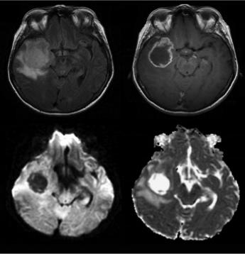
Now, it should be clear that in the case of the destruction of biological barriers such as the cell membranes, ADC should increase as isotropy increases. Hence, it follows that one should expect an increase of ADC in disease as destruction of tissue generally reduces anisotropy. This can be illustrated in Figure 1.8 in a case of a high-grade glioma. The axial T2-FLAIR (a) and T1-weighted post-contrast (b) images demonstrate a right temporal lesion with surrounding edema and ring-shaped enhancement. On the DW image (c), the lesion presents low signal intensity, resulting in high intratumoral ADC (d). The relatively high ADC of the peritumoral edema reflects tumor infiltration in the surrounding parenchyma.
Axis x |
Axis y |
Axis z |
FIGURE 1.7 Three different DW images of a water phantom are depicted, one for each of the principal axes of the scanner, x, y, and z. The lower part of the figure depicts the DW images of the same three principal axis gradients of the scanner for a healthy volunteer.
12 |
Advanced MR Neuroimaging: From Theory to Clinical Practice |
(a) |
(b) |
(c) |
(d) |
FIGURE 1.8 Axial T2-FLAIR (a) and T1-weighted post-contrast (b) images demonstrate a right temporal lesion with surrounding edema and ring-shaped enhancement. On the DW image, the lesion presents low signal intensity (c) resulting in higher intratumoral ADC (d).
1.2.5 Echo Planar Imaging
Since even minimal bulk patient motion during acquisition of DW images can obscure the effects of the much smaller microscopic water motion due to diffusion, fast imaging sequences are necessary for successful clinical DWI. The most widely used DW acquisition technique is single-shot echo-planar imaging (EPI). This is because in a clinical environment, certain requirements are imposed for diffusion studies. First, reasonable imaging time should be achieved (i.e., fast imaging). Second, multiple slices (15–20) are required to cover most of the brain, with good spatial resolution (~3–5 mm thick, 1–3 mm in-plane is required, at a reasonably short TE (120 ms) to reduce T2 decay, and an adequate diffusion sensitivity (ADC ~0.2–1 × 10⁻³ mm2/s for brain tissues). The EPI sequence is fast and insensitive to small motion, which is essential. It is also readily available on most clinical MRI scanners. Because images can be acquired in a fraction of a second, artifacts from patient motion are greatly reduced, and motion between acquisitions with the different required diffusion-sensitizing gradients is also decreased.
Nevertheless, EPI suffers from limitations, which include the limited spatial resolution due to smaller imaging matrices as well as the blurring effect of T2* decay occurring during image readout. Other limitations are sensitivity to artifacts due to magnetic field inhomogeneity, chemical shift effects, ghosting, and local susceptibility effects. The latter is particularly important, as it results in marked distortion and signal drop-out near air cavities, particularly at the skull base and the posterior fossa, limiting sensitivity of DWI with EPI in these areas. Nonetheless, artifacts and pitfalls of DWI are going to be discussed in detail in the next chapter.
Diffusion MR Imaging |
13 |
Alternative DWI techniques include multi-shot EPI with navigator echo correction or DW, periodically rotated overlapping parallel lines with enhanced reconstruction (PROPELLER) and parallel imaging methods, such as sensitivity encoding (SENSE) (Jones et al., 1999; Porter and Mueller, 2004). The application of such techniques increase the bandwidth per voxel in the phase encode direction, thus reducing artifacts arising from field inhomogeneities, like those induced by eddy currents and local susceptibility gradients.
1.2.6 Main Limitations of DWI
DWI is undoubtedly a very useful clinical tool and can help the visual interpretation of clinical images. However, it is only a qualitative type of exam, and is very sensitive to the choice of acquisition parameters and patient motion in the scanner.
Moreover, DWI sequences are sensitive, but not specific for the detection of restricted diffusion. Thus, one should not use only signal changes to quantify diffusion properties, as the signal from DWI is prone to the underlying T2-weighted signal, referred to as the “T2 shinethrough” effect (Chilla et al. 2015). That is, the increased signal in areas of cytotoxic edema on T2-weighted images may be present on the DWI images as well (Jones et al., 1999). To determine whether this signal hyperintensity on DWI images truly represents decreased diffusion, the ADC map should also be used. The ADC sequence is not as sensitive as the DWI sequence for restricted diffusion, but it is more specific; the ADC images are not susceptible to the “T2 shine-through” effect since they are “relative” images (Debnam and Schellingerhout, 2011).
As described above, a typical clinical diffusion imaging protocol consists of four images at each level: (1) one without diffusion weighting (S0), also known as the b = 0 s/mm2 or “b zero” image, which has an image contrast similar to that of a conventional T2-weighted spin-echo image (for echo times and repetition times used in typical diffusion applications) and (2) three images with diffusion weighting along mutually orthogonal directions. For the reasons described earlier, the DW images the radiologist evaluates are not the set of orthogonally weighted images, but rather the geometric mean computed from these three images, also known as the isotropic DW image, or simply the ADC. Hence ADC is equal to
ADC = |
ADC1+ ADC2+ ADC3 |
(1.5) |
|
3 |
|||
|
|
where ADC1, ADC2, and ADC3 are the apparent diffusion coefficients along the directions of the three diffusion-sensitizing gradients. In terms of the acquired signal SDWI in the DW image, we have
SDWI = (S1 × S2 |
× S3)3 |
|
−b |
ADC1 + ADC 2 + ADC3 |
= S0e(−b ADC) |
(1.6) |
|
= S0e |
3 |
|
|||||
|
1 |
|
|
|
|
|
|
An important observation in this last term, is that there are two major sources of contrast in the DW image: the T2-weighted term S0 and the exponential term related to diffusion. Hence, hyperintensity on DWI may be related to T2 prolongation (large S0 term), reduced diffusion, or both. When high signal intensity is observed on DWI due to a dominant T2-related term in the setting of normal or even elevated ADC, it is known as T2 shine-through. Simply examining the b zero image or corresponding conventional T2-weighted image is not a reliable method for differentiating between truly reduced diffusion and T2 shine-through since both prolonged T2 and reduced diffusion may coexist (Pauleit et al., 2004). The T2 shine-through effect of a low-grade glioma is depicted in Figure 1.9.
14 |
Advanced MR Neuroimaging: From Theory to Clinical Practice |
(a) |
(b) |
(c) |
FIGURE 1.9 T2 “shine-through” effect of a low-grade glioma shown on a T2-weighted image (a), which appears bright on the DW image (b) and also bright on the ADC map (c), implying increased diffusivity. (Courtesy Allen D. Elster, MRIquestions.com.)
Unfortunately, ADC suffers from a limitation too. It depends on the direction of the applied diffusion encoding gradient, as was illustrated in Figure 1.7, where it is evident that in certain regions of the brain, ADC is different depending on the applied gradient. This effect, of course, enables us to extract valuable information about the brain microstructure; nevertheless, it also reveals that ADC is directionally dependent (Chenevert et al., 1990; Doran et al., 1990).
In other words, a single ADC would be inadequate for characterizing diffusion in clinical practice as it would depend on the direction of gradients as well as the position and possible movement of the patient’s head. Although in clinical practice the average of the ADC values along the three orthogonal directions is used, known as the mean diffusivity, “trace,” or, simply, the ADC, it is clear that an infinite number of ADC measures can be obtained within anisotropic tissue. This limitation was remedied by a more complex description as the diffusion tensor matrix, which is going to be discussed in detail in the next section.
1.3 Diffusion Tensor Imaging
Focus Point
•ADC is directionally dependent.
•A single ADC is inadequate for characterizing diffusion in vivo.
•Diffusion tensor imaging represents a further development of DWI.
•The diffusion tensor describes an ellipsoid that represents the directional movement of water molecules inside a voxel.
Diffusion tensor imaging (DTI) evolved from DWI and was developed to remedy the limitations of DWI (see previous section), taking advantage of the preferential water diffusion inside the brain tissue (Le Bihan, 2003; Mukherjee, et al., 2008). The water diffusion in the brain is NOT an isotropic process, due to the natural intracellular (neurofilaments and organelles) and extracellular (glial cells and myelin sheaths) barriers that restrict diffusion towards certain directions. Hence, water molecules diffuse mainly along the direction of white matter axons rather than perpendicular to them (please refer to Figure 1.1). Under these circumstances,
Diffusion MR Imaging |
|
15 |
Free diffusion in |
Isotropic diffusion |
Sphere |
isotropic medium |
|
|
|
(a) |
|
Restricted diffusion in |
Anisotropic diffusion |
Ellipsoid |
anisotropic medium |
|
|
(b)
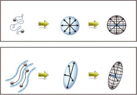
FIGURE 1.10 (a) Free diffusion in an isotropic medium can be represented by a sphere, while restricted diffusion in an anisotropic medium (e.g., inside the white matter fibers) can be represented by an ellipsoid (b).
diffusion can become highly directional along the length of the tract, and is called anisotropic (Price, 2007) (Figure 1.10). This means that we talk about media that have different diffusion properties in different directions. In other words, in certain regions of the brain, ADC is directionally dependent; it is therefore also clear that a single ADC would be inadequate for characterizing diffusion and a more compound mathematical description is required.
In that that sense, DTI measures both the magnitude and the direction of proton movement within a voxel for multiple dimensions of movement using a mathematical model to represent this information, called the diffusion tensor (DT) (Debnam and Schellingerhout, 2011). Assuming that the probability of molecular displacements follows a multivariate Gaussian distribution over the observation diffusion time, the diffusion process can be described by a 3 × 3 tensor matrix, proportional to the variance of the Gaussian distribution. Thus, the diffusion tensor, D, is characterized by nine elements:
|
Dxx |
Dxy |
|
|
|
|
Dxz |
|
|||
|
Dyx |
Dyy |
|
|
(1.7) |
D = |
Dyz |
||||
|
Dzx |
Dzy |
Dzz |
|
|
|
|
|
|
|
|
Now, consider that the directional movement of water molecules inside a voxel can be represented by an ellipsoid (Figure 1.11), which in turn can be described by the tensor in that specific voxel.
This tensor consists of the 3 × 3 matrix derived from diffusivity measurements in at least six different directions. This is because the tensor is diagonally symmetric (Dxy = Dyx, Dyz = Dzy, and Dxz = Dzx), therefore only six unknown elements need to be determined. Figure 1.12 shows the elements of the diffusion tensor. The images of Dxx, Dyy, and Dzz
16 |
Advanced MR Neuroimaging: From Theory to Clinical Practice |
1
v2 v1 2
v3 |
3 |
|
(a) |
(b) |
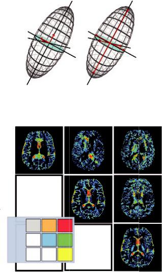
FIGURE 1.11 Three eigenvectors describe the orientation of the three axes of the ellipsoid (a), and three eigenvalues represent the magnitude of the axes (apparent diffusivities) of the ellipsoid (b).
xx |
xy |
xz |
yy |
yz |
6 directions
Dxx |
Dxy |
Dxz |
zz |
D = Dyx |
Dyy |
Dyz |
|
Dzx |
Dzy |
Dzz |
|
FIGURE 1.12 Elements of the diffusion tensor. The images of Dxx, Dyy, and Dzz show the diffusivity along the x-, y-, and z axes, respectively, while the images of Dxy, Dxz, and Dyz show respective displacements in orthogonal directions. Since the tensor is diagonally symmetric (Dxy = Dyx, Dyz = Dzy, and Dxz = Dzx), only six unknown elements need to be determined.
show the diffusivity along the x-, y-, and z axes, respectively, while the images of Dxy, Dxz, and Dyz show respective displacements in orthogonal directions.
If the tensor is completely aligned with the anisotropic medium, then the off-diagonal elements become zero and the tensor is diagonalized. This diagonalization provides three eigenvectors that describe the orientation of the three axes of the ellipsoid, and three eigenvalues, which represent the magnitude of the axes (apparent diffusivities) in the corresponding directions (Figure 1.12). The major axis is considered to be oriented in the direction of maximum diffusivity, which has been shown to coincide with tract orientation (Field and Alexander, 2004; Price, 2007). Therefore, there is a transition through the diffusion tensor from the x, y, z
Diffusion MR Imaging |
17 |
coordinate system defined by the scanner’s geometry, to a new independent coordinate system, in which axes are dictated by the directional diffusivity information.
Depending on the local diffusion, the ellipsoid may be “prolate,” “oblate,” or “spherical.” Prolate shapes are expected in highly organized tracts where the fiber bundles all have similar orientations, oblate shapes are expected when fiber orientations are more variable but remain limited to a single plane, and spherical shapes are expected in areas that allow isotropic diffusion (Alexander et al., 2000).
Going back to our example of ink in the glass of water, over time, the ink particles displace and, because the medium is isotropic, the outer surface of the displacements would resemble a sphere. On the contrary, if water was an anisotropic medium, the ink particles would diffuse preferentially along the principal axis of the anisotropic medium rather than perpendicular to it.
Then, the corresponding displacement profile can no longer be described by a sphere and is more correctly described by an ellipsoid, with the long axis parallel to the long axis of the anisotropic medium as depicted in Figure 1.10.
1.3.1 “Rotationally Invariant” Parameters (Mean
Diffusivity and Fractional Anisotropy)
Using the tensor data, the local diffusion anisotropy can be quantified by the calculation of “rotationally invariant” parameters. The most commonly reported indices that can be calculated are the mean diffusivity (MD) or “Trace” and fractional anisotropy (FA). MD is the mean of the eigenvalues, and represents a directionally measured average of water diffusivity, whereas FA derives from the standard deviation of the three eigenvalues.
More analytically, the trace is the sum of the three diagonal elements of the diffusion tensor (i.e., Dxx + Dyy + Dzz), which can be shown to be equal to the sum of its three eigenvalues. The mean Trace (Trace/3) can be thought of as being equal to the averaged mean diffusivity.
The image of the MD (i.e., trace/3) is depicted in Figure 1.13, which is produced by the average of the ADC indices along the three orthogonal axes (as in Figure 1.7). This averaging produces an evident loss of contrast in parenchyma in the MD map. Nevertheless, Pierpaoli et al. (1996), showed that in the b-value range typically used in clinical studies (b<1500 s/mm2), the MD is fairly uniform throughout parenchyma at a value of about 0.7 × 10⁻³ mm2/s. This is advan tageous in the sense that the effects of anisotropy do not confound the detection of diffusion abnormalities, such as acute ischemic lesions (Lythgoe et al., 1997; Lee et al., 2008). It should be evident, however, that if the b-value is changed, there will be dissociation between white and gray matter (Yoshiura et al., 2001), and moreover, it is obvious that in order to compare results between different institutions the b-value should be the same.
In the same logic, in order to specify a simple but unbiased anisotropy index, Pierpaoli and Basser (1996) came up with the FA and relative anisotropy (RA) indices. These are given by the following equations:
FA = |
3 |
|
(λ1 − λ )2 + (λ2 − λ )2 + (λ3 − λ )2 |
(1.8) |
|
2 |
|
λ12 + λ22 + λ32 |
|
||
and |
|
|
|
|
|
RA = |
1 |
|
(λ1 − λ )2 + (λ2 − λ )2 + (λ3 − λ )2 |
(1.9) |
|
2 |
|
λ |
|
|
|
18 |
Advanced MR Neuroimaging: From Theory to Clinical Practice |
||
|
Axis x |
Axis y |
Axis z |
FIGURE 1.13 Average of the three ADC maps is the mean diffusivity (mathematically equivalent to one third of the trace of the diffusion tensor).
Both parameters indicate how elongated the diffusion ellipsoid is; hence, the information provided is essentially the same, although FA is the parameter most widely used. In an FA map, the signal brightness of a voxel, describes the degree of anisotropy in the given voxel. FA ranges from 0 to 1, depending on the underlying tissue architecture. A value closer to 0 indicates that the diffusion in the voxel is isotropic (unrestricted water movement), such as in areas of CSF, whereas a value closer to 1 describes a highly anisotropic medium, such as in the corpus callosum where water molecules diffuse along a single axis (Price, 2007). Example images showing FA for the whole brain in the axial plane are presented in Figure 1.14.
Diffusion directionality in various regions of interest can be further represented by a directionally encoded color (DEC) FA map as shown in Figure 15d. More specifically, the eigenvector with the largest eigenvalue defines the orientation of the ellipsoid in each voxel, which can then be color-coded to evaluate and display information about the direction of white matter tracts. Hence, ellipsoids describing diffusion from left to right are red (x-axis), ellipsoids describing anterioposterior (y-axis) diffusion are green, and diffusion in the craniocaudal direction is blue (z-axis) (Pajevic and Pierpaoli, 1999). This procedure provides a user friendly and convenient summary map from which one can determine the degree of anisotropy (in terms of signal brightness) and the fiber orientation in the voxel (in terms of hue). A neuroradiologist can then combine and correlate this information with normal brain anatomy, identify specific white matter tracts, and assess the impact of a lesion on neighboring white matter fibers (Ferda et al., 2010). Figure 1.15 depicts the comparison of a T2-weighted, average diffusion coefficient (DC), fractional anisotropy (FA) map, and colorcoded orientation map.
Diffusion MR Imaging |
19 |
FIGURE 1.14 Example images showing FA for the whole brain in the axial plane. Directionally DEC FA map.
(a) |
(b) |
(c) |
(d) |
FIGURE 1.15 Comparison of T2-weighted (a), average diffusion coefficient (DC) (b), fractional anisotropy (FA) map (c), and color-coded orientation map (d). Images were acquired using a 3.0 T scanner. The colors represent the orientations of fibers; red: right–left, green: anterior–posterior, and blue: superior–inferior.
1.3.2 Fiber Tractography
By now, it must be evident that the underlying tissue structure dictates diffusion anisotropy, and in the human brain, this is mainly the white matter architecture. Hence, by combining FA values with directionality, it would be possible to obtain estimates of fiber orientation. This idea has led to the development of fiber tractography enabling the mapping of white matter tracts noninvasively (Westin et al., 2002; Assaf and Pasternak, 2008), as seen in Figure 1.16.
20 |
Advanced MR Neuroimaging: From Theory to Clinical Practice |
FIGURE 1.16 MR fiber tractography.
FIGURE 1.17 Schematic diagram of the line propagation approach.
Different algorithms have been developed for fiber tractography, but the main idea is that following the tensor’s orientation on a voxel-by-voxel basis, it is possible to identify intravoxel connections and display specific fiber tracts using computer graphic techniques (Figure 1.17). A variety of tractography techniques have been reported (Jones et al., 1999; Mori et al., 1999; Mori et al., 2002, Parker et al., 2002). All these techniques use mathematical models to identify neighboring voxels that might be located within the same fiber tract based on the regional tensor orientations and relative positions of the voxels.
Towards this direction, a number of studies have created atlases of the human brain based on DTI and tractography (Jellison et al., 2004; Wakana et al., 2004; Mori et al., 2009). According to this, a very important differential diagnostic parameter regarding the displacement or disruption
Diffusion MR Imaging |
21 |
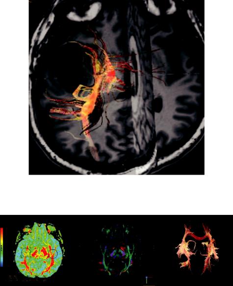
of a specific fiber tract by a pathology may be assessed by 3D tractograms (Bello et al., 2010; Mori and Zijl, 2002), as is displayed in a case of brain tumor tractography in Figure 1.18.
In order to produce tracts, the user needs to define a “seed” region of interest (ROI) on the color orientation map that is very useful in visualizing the white matter tract orientation. In most software applications, this is defined as “Structural View.” Depositing a seed ROI results in a white matter track oriented through the ROI. To display white matter tracks oriented from one ROI to another ROI, one needs to position a second ROI on the image and define a “target” ROI. This is illustrated in Figure 1.19.
FIGURE 1.18 Displacement or disruption of a specific fiber tract by a pathology may be assessed by 3D tractograms.
(a) |
(b) |
(c) |
FIGURE 1.19 FA map (a), ROI placement on colored orientation map (b), and fiber tracts (c).
22 |
Advanced MR Neuroimaging: From Theory to Clinical Practice |
FIGURE 1.20 Spinal cord diffusion tensor tractography. (Courtesy of General Electric, with permission, and Mt. Sinai Hospital.)
These techniques also provide useful information in terms of presurgical planning (Romano et al., 2009; Arfanakis et al., 2006). Nonetheless, they present limitations such as in cases of complex tracts (crossing or branching fibers), which should be taken into consideration when these methods are used for preoperative guidance (Jones, 2010).
In DTI, the diffusion gradients are applied in multiple directions, and based on previous reports, the number of non-collinear gradients applied varies (ranging from 6 to 55). There is much debate in the literature; however, an optimal number has not yet been defined (Hasan et al., 2001; Jones, 2004; Nucifora et al., 2007). As one can imagine, the main drawback of an increased number of gradients in DTI is the imaging time, which increases simultaneously and may not be applicable in clinical practice (Gupta et al., 2010). Therefore, as always, there is a trade-off between the imaging time and the number of gradients applied in order to obtain sufficient diffusion information.
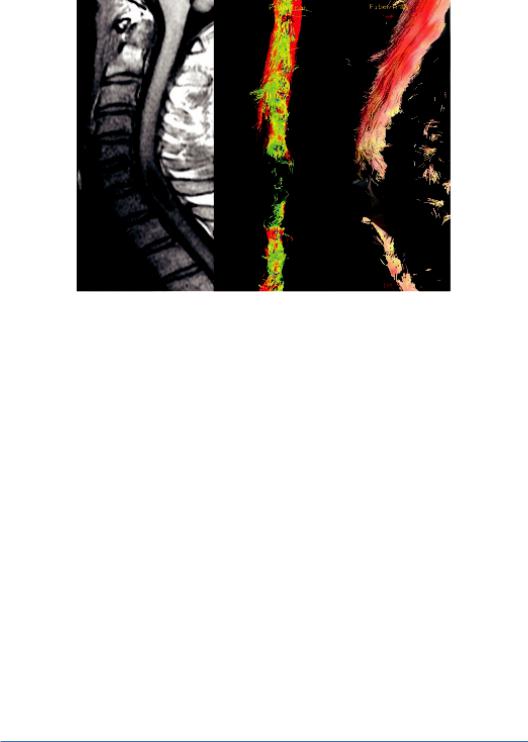
DTI has also been applied in the spinal cord, in the evaluation of acute and chronic trauma, tumors of the spinal canal, degenerative myelopathy, demyelinating and infectious diseases, and so on, and there are strong indications that it can be a sensitive and specific method (Jones et al., 1999). Figure 1.20 illustrates a case of spinal cord diffusion tensor tractography.
It has to be noted that there are still many technical limitations in the application of spinal cord DTI, especially in thoracic and lumbar segments. Nevertheless, the wider use of higher field scanners (3T or more), and the further development of acquisition and post-processing techniques, should result in the increased role of this promising advanced technique in both research and clinical practice.
1.4 Conclusions and Future Perspectives
The usefulness of conventional MRI in the detection of cerebral pathology has been wellestablished, although it can be in many cases nonspecific despite the excellent soft tissue visualization. The addition of DWI and DTI has truly revolutionized clinical neuroimaging,

Diffusion MR Imaging |
23 |
providing microstructural information with specific benefits, which can be summarized in the following points:
1.Pathology may be detected earlier and in a quantitative manner, allowing increased specificity.
2.The microarchitecture of the brain can now be deeply explored.
3.DWI/DTI metrics can be used as quantifiable objective features allowing tumor classification as well as treatment monitoring.
4.Diffusion may aid the differentiation between cytotoxic brain edema (restricted diffusion) and vasogenic edema (increased diffusion) offering both diagnostic (tumor categorization) and prognostic (reversible pathology) value.
5.The functional connectivity within the brain is now explored using DTI to evaluate white matter tracts. Besides clinical studies, this is expected to optimize surgery planning and therefore treatment outcome.
Moreover, a number of significant future clinical applications will emerge, as there is intensive ongoing research in the field with increasing applications, which will be translated into routine clinical neuroimaging. Based on the aforementioned points, it is expected that the diagnosis of several pathologies such as ischemia, infection, and demyelinating disease will benefit as well.
Nevertheless, caution against over-reliance on “scientific extras” and “advanced tools” is needed since we must never forget that even as sophisticated a mathematic construct as the DTI model is, it is an oversimplification of the properties of water diffusion in the brain, with several associated limitations.
These limitations mainly involve the complex white matter architecture with kissing, branching and intersecting fiber tracts, which may result in erroneous estimation of the white matter tracks, as well as in problematic evaluation of diffusion indices like FA or MD.
The limitations of DWI/DTI techniques with their associated artifacts and pitfalls that one should take into account are going to be analytically discussed in the next chapter.
References
Alexander, A. L., Hasan, K., Kindlmann, G., Parker, D. L., and Tsuruda, J. S. (2000). A geometric analysis of diffusion tensor measurements of the human brain. Magnetic Resonance in Medicine, 44(2), 283–291. doi:10.1002/1522-2594(200008)44:2<283::aid-mrm16>3.0.co;2-v Arfanakis, K., Gui, M. and Lazar, M. (2006). Optimization of white matter tractography for pre-surgical planning and image-guided surgery. Oncology Reports, 15 Spec no., 1061–1064.
10.3892/or.15.4.1061.
Assaf, Y. and Basser, P. J. (2005). Composite hindered and restricted model of diffusion (CHARMED) MR imaging of the human brain. NeuroImage, 27(1), 48–58. doi:10.1016/ j.neuroimage.2005.03.042">10.1016/j.neuroimage.2005.03.042
Assaf, Y. and Pasternak, O. (2008). Diffusion tensor imaging (DTI)-based white matter mapping in brain research: A review. Journal of Molecular Neuroscience, 34(1), 51–61. https://doi. org/10.1007/s12031-007-0029-0
Beaulieu, C. (2002). The basis of anisotropic water diffusion in the nervous system—A technical review. NMR in Biomedicine, 15(7–8), 435–455. doi:10.1002/nbm.782
Beaulieu, C. and Allen, P. S. (1994a). Determinants of anisotropic water diffusion in nerves. Magnetic Resonance in Medicine, 31(4), 394–400. doi:10.1002/mrm.1910310408
24 |
Advanced MR Neuroimaging: From Theory to Clinical Practice |
Beaulieu, C. and Allen, P. S. (1994b). Water diffusion in the giant axon of the squid: Implications for diffusion-weighted MRI of the nervous system. Magnetic Resonance in Medicine, 32(5), 579–583. doi:10.1002/mrm.1910320506
Beaulieu, C. and Allen, P. S. (1996). An in vitro evaluation of the effects of local magnetic-sus- ceptibility-induced gradients on anisotropic water diffusion in nerve. Magnetic Resonance in Medicine, 36(1), 39–44. doi:10.1002/mrm.1910360108
Bello, L., Castellano, A., Fava, E., Casaceli, G., Riva, M., Scotti, G. et al. (2010). Intraoperative use of diffusion tensor imaging fiber tractography and subcortical mapping for resection of gliomas: Technical considerations. Neurosurgical Focus, 28(2). doi:10.3171/2009.12. focus09240
Ben-Amitay, S., Jones, D. K., and Assaf, Y. (2012). Motion correction and registration of high b-value diffusion weighted images. Magnetic Resonance in Medicine, 67(6), 1694–1702. doi:10.1002/mrm.23186
Bloch, F. (1950). Nuclear induction. Physics Today, 3(8), 22–25. doi:10.1063/1.3066970 Chenevert, T. L., Brunberg, J. A., and Pipe, J. G. (1990). Anisotropic diffusion in human white
matter: Demonstration with MR techniques in vivo. Radiology, 177(2), 401–405. doi:10.1148/ radiology.177.2.2217776
Chilla, G. S., Tan, C. H., Xu, C., and Poh, C. L. (2015). Diffusion weighted magnetic resonance imaging and its recent trend—A survey. Quantitative Imaging in Medicine and Surgery,
5(3), 407–422. http://doi.org/10.3978/j.issn.2223-4292.2015.03.01
Debnam, J. M. and Schellingerhout, D. (2011). Diffusion MR imaging of the brain in patients with cancer. International Journal of Molecular Imaging, 2011, 1–9. doi:10.1155/2011/714021
Doran, M., Hajnal, J. V., Bruggen, N. V., King, M. D., Young, I. R., and Bydder, G. M. (1990). Normal and Abnormal White Matter Tracts Shown by MR Imaging using Directional Diffusion Weighted Sequences. Journal of Computer Assisted Tomography, 14(6), 865–873. doi:10.1097/00004728-199011000-00001
Einstein, A. (1905). Über die von der molekularkinetischen Theorie der Wärme geforderte Bewegung von in ruhenden Flüssigkeiten suspendierten Teilchen. Annalen der Physik, 322(8), 549–560. doi:10.1002/andp.19053220806
Fan, G. G., Deng, Q. L., Wu, Z. H., and Guo, Q. Y. (2006). Usefulness of diffusion/perfusionweighted MRI in patients with non-enhancing supratentorial brain gliomas: A valuable tool to predict tumour grading? The British Journal of Radiology, 79(944), 652–658. doi:10.1259/bjr/25349497
Ferda, J., Kastner, J., Mukenšnabl, P., Choc, M., Horemužová, J., Ferdová, E., and Kreuzberg, B. (2010). Diffusion tensor magnetic resonance imaging of glial brain tumors. European Journal of Radiology, 74(3), 428–436. doi:10.1016/j.ejrad.2009.03.030
Field, A. S. and Alexander, A. L. (2004). Diffusion tensor imaging in cerebral tumor diagnosis and therapy. Topics in Magnetic Resonance Imaging, 15(5), 315–324. doi:10.1097/ 00002142-200410000-00004
Gillard, J. H., Waldman, A. D., and Barker, P. B. (2005). Clinical MR Neuroimaging: Physiological and functional techniques. Cambridge: Cambridge University Press.
Guo, A. C., Macfall, J. R., and Provenzale, J. M. (2002). Multiple sclerosis: Diffusion tensor MR imaging for evaluation of normal-appearing white matter. Radiology, 222(3), 729–736. doi:10.1148/radiol.2223010311
Gupta, A., Holodny, A. I., Shah, A., and Young, R. J. (2010). Imaging of brain tumors: Functional magnetic resonance imaging and diffusion tensor imaging. Neuroimaging Clinics of North America, 20(3), 379–400.
Diffusion MR Imaging |
25 |
Hahn, E. L. (1950). Spin echoes. Physical Review, 80(4), 580–594. doi:10.1103/physrev.80.580 Hakyemez, B., Erdogan, C., Gokalp, G., Dusak, A., and Parlak, M. (2010). Solitary metasta-
ses and high-grade gliomas: Radiological differentiation by morphometric analysis and perfusion-weighted MRI. Clinical Radiology, 65(1), 15–20. doi:10.1016/j.crad.2009.09.005
Hasan, K. M., Parker, D. L., and Alexander, A. L. (2001). Comparison of gradient encoding schemes for diffusion-tensor MRI. Journal of Magnetic Resonance Imaging, 13(5), 769–780. doi:10.1002/jmri.1107
Hong, X. and Dixon, W. T. (1992). Measuring diffusion in inhomogeneous systems in imaging mode using antisymmetric sensitizing gradients. Journal of Magnetic Resonance (1969), 99(3), 561–570. doi:10.1016/0022-2364(92)90210-x
Jellison, B. J., Alexander, A. L., Field, A. S., Lazar, M., Medow, J., and Salamat, M. S. (2004). Diffusion tensor imaging of cerebral white matter: A pictorial review of physics, fiber tract anatomy, and tumor imaging patterns. AJNR American journal of neuroradiology, 25(3), 356–369.
Jones, D., Horsfield, M., and Simmons, A. (1999). Optimal strategies for measuring diffusion in anisotropic systems by magnetic resonance imaging. Magnetic Resonance in Medicine, 42(3), 515–525. doi:10.1002/(SICI)1522-2594(199909)42:3<515::AID-MRM14>3.0.CO;2-Q Jones, D. K. (2004). The effect of gradient sampling schemes on measures derived from diffusion tensor MRI: A Monte Carlo study. Magnetic Resonance in Medicine, 51(4), 807–815.
doi:10.1002/mrm.20033
Jones, D. K. (2010). Challenges and limitations of quantifying brain connectivity in vivo with diffusion MRI. Imaging in Medicine, 2(3), 341–355. doi:10.2217/iim.10.21
Jones, D. K., Knösche, T. R., and Turner, R. (2013). White matter integrity, fiber count, and other fallacies: The do’s and don’ts of diffusion MRI. NeuroImage, 73, 239–254. doi:10.1016/j. neuroimage.2012.06.081
Jones, D. K., Simmons, A., Williams, S. C., and Horsfield, M. A. (1999). Non-invasive assessment of axonal fiber connectivity in the human brain via diffusion tensor MRI. Magnetic Resonance in Medicine, 42(1), 37–41. doi:10.1002/(sici)1522-2594(199907)42:1<37::aid- mrm7>3.0.co;2-o
Kaden, E., Kelm, N. D., Carson, R. P., Does, M. D., & Alexander, D. C. (2016). Multi-compartment microscopic diffusion imaging. NeuroImage, 139, 346–359. doi:10.1016/j.neuroimage. 2016.06.002
Kono, K., Inoue, Y., Morino, M., Nakayama, K., Ohata, K., Shakudo, M., Wakasa, K., and Yamada, R. (2001). The role of diffusion-weighted imaging in patients with brain tumors.
AJNR American Journal of Neuroradiology, 22(6), 1081–1088.
Lam, W., Poon, W., and Metreweli, C. (2002). Diffusion MR imaging in glioma: Does it have any role in the pre-operation determination of grading of glioma? Clinical Radiology, 57(3), 219– 225. doi:10.1053/crad.2001.0741
Le Bihan, D. (2003). Looking into the functional architecture of the brain with diffusion MRI. Nature Reviews Neuroscience, 4(6), 469–480. doi:10.1038/nrn1119
Le Bihan, D., Breton, E., Lallemand, D., Grenier, P., Cabanis, E., and Laval-Jeantet, M. (1986). MR imaging of intravoxel incoherent motions: Application to diffusion and perfusion in neurologic disorders. Radiology, 161(2), 401–407. doi:10.1148/radiology.161.2.3763909
Le Bihan, D., Poupon, C., Amadon, A., and Lethimonnier, F. (2006). Artifacts and pitfalls in diffusion MRI. Journal of Magnetic Resonance Imaging, 24(3), 478–488. doi:10.1002/ jmri.20683
Lee, H. Y., Na, D. G., Song, I., Lee, D. H., Seo, H. S., Kim, J., and Chang, K. (2008). Diffusiontensor imaging for glioma grading at 3-T magnetic resonance imaging. Journal of Computer Assisted Tomography, 32(2), 298–303. doi:10.1097/rct.0b013e318076b44d
26 |
Advanced MR Neuroimaging: From Theory to Clinical Practice |
Lian, J., Williams, D., and Lowe, I. (1994). Magnetic resonance imaging of diffusion in the presence of background gradients and imaging of background gradients. Journal of Magnetic Resonance, Series A, 106(1), 65–74. doi:10.1006/jmra.1994.1007
Lythgoe, M. F., Busza, A. L., Calamante, F., Sotak, C. H., King, M. D., Bingham, A. C., and Gadian, D. G. (1997). Effects of diffusion anisotropy on lesion delineation in a rat model of cerebral ischemia. Magnetic Resonance in Medicine, 38(4), 662–668. doi:10.1002/ mrm.1910380421
Mori, S., Crain, B. J., Chacko, V. P., and Zijl, P. C. (1999). Three-dimensional tracking of axonal projections in the brain by magnetic resonance imaging. Annals of Neurology, 45(2), 265–269. doi:10.1002/1531-8249(199902)45:2<265::aid-ana21>3.0.co;2–3
Mori, S., Frederiksen, K., Zijl, P. C., Stieltjes, B., Kraut, M. A., Solaiyappan, M., and Pomper, M. G. (2002). Brain white matter anatomy of tumor patients evaluated with diffusion tensor imaging. Annals of Neurology, 51(3), 377–380. doi:10.1002/ana.10137
Mori, S., Oishi, K., and Faria, A. V. (2009). White matter atlases based on diffusion tensor imaging. Current Opinion in Neurology, 22(4), 362–369. http://doi.org/10.1097/WCO. 0b013e32832d954b
Mori, S. and Zijl, P. C. (2002). Fiber tracking: Principles and strategies—A technical review. NMR in Biomedicine, 15(7–8), 468–480. doi:10.1002/nbm.781
Moritani, T., Ekholm, S., and Westesson, P. (2009). Diffusion-Weighted MR Imaging of the Brain. Berlin: Springer.
Mukherjee, P., Berman, J., Chung, S., Hess, C., and Henry, R. (2008). Diffusion tensor MR imaging and fiber tractography: Theoretic underpinnings. American Journal of Neuroradiology, 29(4), 632–641. doi:10.3174/ajnr.a1051
Nagar, V., Ye, J., Ng, W., Chan, Y., Hui, F., Lee, C., and Lim, C. (2008). Diffusion-weighted MR imaging: diagnosing atypical or malignant meningiomas and detecting tumor dedifferentiation. American Journal of Neuroradiology, 29(6), 1147–1152. doi:10.3174/ajnr.a0996
Nucifora, P. G., Verma, R., Lee, S., and Melhem, E. R. (2007). Diffusion-tensor MR imaging and tractography: Exploring brain microstructure and connectivity. Radiology, 245(2), 367–384. doi:10.1148/radiol.2452060445
Pajevic, S. and Pierpaoli, C. (1999). Color schemes to represent the orientation of anisotropic
tissues from diffusion tensor data: Application to white matter fiber tract mapping in the human brain. Magnetic Resonance in Medicine, 42(3), 526–540. doi:10.1002/ (sici)1522-2594(199909)42:3<526::aid-mrm15>3.3.co;2-a
Parker, G. J., Stephan, K. E., Barker, G. J., Rowe, J. B., Macmanus, D. G., Wheeler-Kingshott, C. A. et al. (2002). Initial demonstration of in vivo tracing of axonal projections in the macaque brain and comparison with the human brain using diffusion tensor imaging and fast marching tractography. NeuroImage, 15(4), 797–809. doi:10.1006/nimg.2001.0994
Pauleit, D., Langen, K., Floeth, F., Hautzel, H., Riemenschneider, M. J., Reifenberger, G., and Müller, H. (2004). Can the apparent diffusion coefficient be used as a noninvasive parameter to distinguish tumor tissue from peritumoral tissue in cerebral gliomas? Journal of Magnetic Resonance Imaging, 20(5), 758–764. doi:10.1002/jmri.20177
Pierpaoli, C. and Basser, P. J. (1996). Toward a quantitative assessment of diffusion anisotropy. Magnetic Resonance in Medicine, 36(6), 893–906. doi:10.1002/mrm.1910360612
Pierpaoli, C., Jezzard, P., Basser, P. J., Barnett, A., and Chiro, G. D. (1996). Diffusion tensor MR imagingofthehumanbrain.Radiology,201(3),637–648.doi:10.1148/radiology.201.3.8939209
Diffusion MR Imaging |
27 |
Porter, D. and Mueller, E. (2004). Multi-shot diffusion-weighted EPI with readout mosaic segmentation and 2D navigator correction. Proceedings of the 12th Annual Meeting of ISMRM, 11, 442.
Price, S. J. (2007). The role of advanced MR imaging in understanding brain tumour pathology. British Journal of Neurosurgery, 21(6), 562–575. doi:10.1080/02688690701700935
Romano, A., D’Andrea, G., Minniti, G., Mastronardi, L., Ferrante, L., Fantozzi, L. M., and Bozzao, A. (2009). Pre-surgical planning and MR-tractography utility in brain tumour resection. European Radiology, 19(12), 2798-2808. doi:10.1007/s00330-009-1483-6
Schellinger, P. D., Fiebach, J. B., Jansen, O., Ringleb, P. A., Mohr, A., Steiner, T. et al. (2001). Stroke magnetic resonance imaging within 6 hours after onset of hyperacute cerebral ischemia. Annals of Neurology, 49(4), 460–469. doi:10.1002/ana.95.abs
Schmainda, K. M. (2012). Diffusion-weighted MRI as a biomarker for treatment response in glioma. CNS Oncology, 1(2), 169–180. doi:10.2217/cns.12.25
Seo, H., Chang, K., Na, D., Kwon, B., and Lee, D. (2008). High b-value diffusion (b = 3000 s/ mm2) MR imaging in cerebral gliomas at 3T: Visual and quantitative comparisons with b = 1000 s/mm2. American Journal of Neuroradiology, 29(3), 458–463. doi:10.3174/ajnr.a0842
Stejskal, E. O. and Tanner, J. E. (1965). Spin diffusion measurements: Spin echoes in the presence of a time dependent field gradient. Journal of Chemical Physics, 42(1), 288–292. doi:10.1063/1.1695690
Tanner, J. E. (1978). Transient diffusion in a system partitioned by permeable barriers. Application to NMR measurements with a pulsed field gradient. Journal of Chemical Physics, 69(4), 1748–1754. doi:10.1063/1.436751
Thomsen, C., Henriksen, O., and Ring, P. (1987). In vivo measurement of water self diffusion in the human brain by magnetic resonance imaging. Acta Radiologica, 28(3), 353–361. doi:10.1177/028418518702800324
Toh, C., Castillo, M., Wong, A., Wei, K., Wong, H., Ng, S., and Wan, Y. (2008b). Primary cerebral lymphoma and glioblastoma multiforme: Differences in diffusion characteristics evaluated with diffusion tensor imaging. American Journal of Neuroradiology, 29(3), 471–475. doi:10.3174/ajnr.a0872
Wakana, S., Jiang, H., Nagae-Poetscher, L. M., Zijl, P. C., and Mori, S. (2004). Fiber tract– based atlas of human white matter anatomy. Radiology, 230(1), 77–87. doi:10.1148/ radiol.2301021640
Westin, C., Maier, S., Mamata, H., Nabavi, A., Jolesz, F., and Kikinis, R. (2002). Processing and visualization for diffusion tensor MRI. Medical Image Analysis, 6(2), 93–108. doi:10.1016/ s1361-8415(02)00053-1
Yamasaki, F., Kurisu, K., Satoh, K., Arita, K., Sugiyama, K., Ohtaki, M. et al. (2005). Apparent diffusion coefficient of human brain tumors at MR imaging. Radiology, 235(3), 985–991. doi:10.1148/radiol.2353031338
Yoshiura, T., Wu, O., Zaheer, A., Reese, T. G., and Sorensen, A. G. (2001). Highly diffusionsensitized MRI of brain: Dissociation of gray and white matter. Magnetic Resonance in Medicine, 45(5), 734–740. doi:10.1002/mrm.1100
Zakaria, R., Das, K., Radon, M., Bhojak, M., Rudland, P. R., Sluming, V., and Jenkinson, M. D. (2014). Diffusion-weighted MRI characteristics of the cerebral metastasis to brain boundary predicts patient outcomes. BMC Medical Imaging, 14(1), 26. doi:10.1186/1471-2342-14-26