

From the Formal Concept Analysis to the Numerical Simulation … |
117 |
|
|
|
40 |
|
|
|
|
|
|
|
|
|
|
|
|
|
|
|
|
|
|
|
|
|
50 |
(dB) |
0 |
|
|
|
|
|
|
|
|
|
10 |
|
|
|
|
|
|
|
|
|
|
||
-40 |
|
|
|
|
|
|
|
|
|
5 |
|
|
|
|
|
|
|
|
|
|
|
||
Gain |
|
|
|
|
|
|
|
|
|
0 |
|
|
|
|
|
|
|
|
|
|
|
||
-80 |
|
|
|
|
|
|
|
|
|
|
|
|
|
|
|
|
|
|
|
|
|
|
|
|
-120 |
-7 |
-6 |
-5 |
-4 |
-3 |
-2 |
-1 |
0 |
1 |
2 |
|
10 |
10 |
10 |
10 |
10 |
10 |
10 |
10 |
10 |
10 |
|
|
0 |
|
|
|
|
|
|
|
|
|
|
|
|
|
50 |
|
|
|
|
|
|
|
|
(deg) |
-45 |
|
10 |
|
|
|
|
|
|
|
|
|
5 |
|
|
|
|
|
|
|
|
||
|
|
|
|
|
|
|
|
|
|
||
Phase |
|
|
0 |
|
|
|
|
|
|
|
|
-90 |
|
|
|
|
|
|
|
|
|
|
|
|
|
|
|
|
|
|
|
|
|
|
|
|
-135 |
-7 |
-6 |
-5 |
-4 |
-3 |
-2 |
-1 |
0 |
1 |
2 |
|
10 |
10 |
10 |
10 |
10 |
10 |
10 |
10 |
10 |
10 |
|
|
|
|
|
|
|
Frequency (rad/s) |
|
|
|
|
|
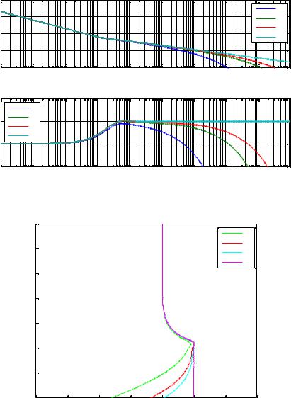
Figure 18. Bode diagrams of ( |
) for |
* |
+ |
Gain (dB)
40 |
|
|
|
|
|
|
|
|
|
|
|
|
|
|
50 |
20 |
|
|
|
|
|
|
10 |
|
|
|
|
|
|
5 |
|
|
|
|
|
|
|
|
|
|
|
|
|
|
|
|
0 |
0 |
|
|
|
|
|
|
|
-20 |
|
|
|
|
|
|
|
-40 |
|
|
|
|
|
|
|
-60 |
|
|
|
|
|
|
|
-80 |
|
|
|
|
|
|
|
-100 |
|
|
|
|
|
|
|
-270 |
-225 |
-180 |
-135 |
-90 |
-45 |
0 |
45 |
Phase (deg)
Figure 19. Black-Nichols plots of ( |
) for |
* |
+ |
. |
7. Simulink Responses
In this last part of the chapter, the Simulink responses will be presented for both the semiinfinite and the finite aluminum media. For both cases, the exact system is implemented on
Simulink.
So, Figure 20 shows the Simulink system whereas Figure 21 represents the temperature variation with respect to time for different values of the sensor placement.
Complimentary Contributor Copy

118 |
Riad Assaf, Roy Abi Zeid Daou, Xavier Moreau et al. |
|
|
|
Time |
|
Clock |
To Workspace |
Scope4 |
|
|
Scope1 |
|
|
|
|
|
|
|
1 |
sqrt(u[1]) |
|
|
|
|
|
|
s |
|
|
|
|
|
|
|
|
|
|
|
|
|
|
|
Transfer Fcn2 |
Fcn1 |
|
Dot Product |
|
|
|
|
|
|
|
|
|
|
1 |
|
U1 |
H0(1) |
|
|
|
|
|
|
|
|
|
|
||
Constant |
Step1 |
Gain3 |
Gain1 |
|
|
Dot Product1 |
|
|
|
|
|
||||
|
|
wx(1) |
1 |
f(u) |
exp(-(u[1])) |
|
Temp |
|
|
s |
|
||||
|
|
|
|
|
|
To Workspace1 |
|
|
|
Gain2 |
Transfer Fcn |
Fcn3 |
Fcn2 |
Scope |
Figure 20. Simulink representation for the semi-infinite homogeneous plane.
|
0.8 |
|
|
|
|
|
|
|
|
|
|
|
|
|
|
|
|
|
|
|
|
|
0 |
|
0.7 |
|
|
|
|
|
|
|
|
|
1 |
|
|
|
|
|
|
|
|
|
|
|
|
|
|
|
|
|
|
|
|
|
|
|
5 |
|
0.6 |
|
|
|
|
|
|
|
|
|
10 |
|
|
|
|
|
|
|
|
|
|
50 |
|
(°C) |
|
|
|
|
|
|
|
|
|
|
|
|
|
|
|
|
|
|
|
|
|
100 |
|
Variation |
0.5 |
|
|
|
|
|
|
|
|
|
|
0.4 |
|
|
|
|
|
|
|
|
|
|
|
Temperature |
|
|
|
|
|
|
|
|
|
|
|
0.3 |
|
|
|
|
|
|
|
|
|
|
|
|
|
|
|
|
|
|
|
|
|
|
|
|
0.2 |
|
|
|
|
|
|
|
|
|
|
|
0.1 |
|
|
|
|
|
|
|
|
|
|
|
0 |
0 |
10 |
20 |
30 |
40 |
50 |
60 |
70 |
80 |
90 |
|
|
|
|
|
Time (s), T0=0°C, Flux=2000W/m2 |
|
|
|
|||
Figure 21. Step responses of ( ) using Simulink for |
* |
+ |
. |
Note that, when comparing Figure 6 to Figure 21, a small time variation of about appears due to the simulation time needed in Simulink that didn’t show up when
using Matlab.
As for the finite medium, Figure 22 and Figure 23 show the Simulink system and the temperature variation with respect to time for different values of the sensor placement and for two values of :
- |
for Figure 23a, |
is equal to |
|
- |
for Figure 23b, |
is equal to |
. |
Complimentary Contributor Copy
|
|
|
|
|
|
|
|
From the Formal Concept Analysis to the Numerical Simulation … |
119 |
|||||||||||||||||||||||||||||||||||||||||||||||||||||||||||
|
|
|
|
|
|
|
|
|
|
|
|
|
|
|
|
|
|
|
|
|
|
|
|
|
|
|
|
|
|
|
|
|
|
|
|
|
|
|
|
|
|
|
|
|
|
|
|
|
|
|
|
|
|
|
|
|
|
|
|
|
|
|
|
|
|
|
|
|
|
|
|
|
|
|
|
|
|
|
|
|
|
|
|
|
|
|
|
|
|
|
|
|
|
|
|
|
|
|
|
|
|
|
|
|
|
|
|
|
|
|
|
|
|
|
|
|
|
|
|
|
|
|
|
|
|
|
|
|
|
|
|
|
|
|
|
|
|
|
|
|
|
|
|
|
|
|
|
|
|
|
|
|
|
|
|
|
|
|
|
|
|
|
|
|
|
|
|
|
|
|
|
|
|
|
|
|
|
|
|
|
|
|
|
|
|
|
|
|
|
|
|
Time |
|
|
|
|
|
|
|
|
|
|
|
|||
|
|
|
|
|
|
|
|
|
|
|
|
|
|
|
|
|
|
|
|
|
|
|
|
|
|
|
|
|
|
|
|
|
|
|
|
|
|
|
|
|
|
|
|
|
|
|
|
|
|
|
|
|
|
|
|
|
|
|
|
|
|
|
|
|||||
|
|
|
|
|
|
|
|
|
|
|
|
|
|
|
|
|
|
|
|
|
|
|
|
|
|
|
|
|
|
|
|
|
|
|
|
|
|
|
|
|
|
Clock |
|
|
|
|
|
|
|
|
|
|
|
|
||||||||||||||
|
|
|
|
|
|
|
|
|
|
|
|
|
|
|
|
|
|
|
|
|
|
|
|
|
|
|
|
|
|
|
|
|
|
|
|
|
|
|
|
|
|
|
|
|
|
|
|
|
|
|
|
|
|
|
|
|
|
|
||||||||||
|
|
|
|
|
|
|
|
|
|
|
|
|
|
|
|
|
|
|
|
|
|
|
|
|
|
|
|
|
|
|
|
|
|
|
|
|
|
To Workspace |
|
|
|
|
|
|
|
|
||||||||||||||||||||||
|
|
|
|
|
|
|
wLx |
|
|
|
|
1 |
|
|
|
|
|
|
power(u[1],-0.5) |
|
|
cosh(u[1]) |
|
|
|
|
|
|
|
|
|
|
|
|
|
|
|
|
|
Scope4 |
||||||||||||||||||||||||||||
|
|
|
|
|
|
|
|
|
|
|
|
|
s |
|
|
|
|
|
|
|
|
|
|
|
|
|
|
|
|
|
|
|
|
|
|
|
|
|
|
|
|
|
|
|
||||||||||||||||||||||||
|
|
|
|
|
|
|
|
|
|
|
|
|
|
|
|
|
|
|
|
|
|
|
|
|
|
|
|
|
|
|
|
|
|
|
|
|
|
|
|
|
|
|
|
|
|
|
|
|
|
|
|
|
|
|
|
|
|
|
|
|
|
|
|
|
|
|
|
|
|
|
|
|
|
|
|
|
|
|
|
|
|
|
|
|
|
|
|
|
|
|
|
|
|
|
|
|
|
|
|
|
|
|
|
|
|
|
|
|
|
|
|
|
|
|
|
|
|
|
|
|
|
|
|
|
|
|
|
|
|
|
|
|
|
|
|
|
|
|
|
|
|
|
|
|
|
Gain3 |
|
Transfer Fcn2 |
|
|
|
|
|
|
Fcn4 |
|
Fcn6 |
|
|
|
|
|
|
|
|
|
|
|
|
|
|
|
|
|
|
|
|
|
|
|
|
|
|
|
|
|
|
|
|
|||||||||||||||||
|
|
|
|
|
|
|
|
|
|
|
|
1 |
|
|
|
|
|
|
|
|
|
|
|
|
|
|
|
|
|
|
|
|
|
|
|
|
|
|
|
|
|
|
|
|
|
|
|
|
|
|
|
|
|
|
|
|
|
|
|
|
|
|
|
|
|
|||
|
|
|
|
|
|
|
|
|
|
|
|
|
|
|
|
|
|
|
|
|
|
|
|
|
|
|
|
|
|
|
|
|
|
|
|
|
|
|
|
|
|
|
|
|
|
|
|
|
|
|
|
|
|
|
|
|
|
|
|
|
|
|
|
|||||
|
|
|
|
|
|
|
|
|
|
|
|
|
|
|
|
|
|
|
|
|
|
|
|
|
|
|
|
|
|
|
|
|
|
|
|
|
|
|
|
|
|
|
|
|
|
|
|
|
|
|
|
|
|
|
|
|
|
|
|
|
|
|
|
|||||
|
|
|
|
|
|
|
wL |
|
|
|
|
|
|
|
|
power(u[1],-0.5) |
|
|
1/cosh(u[1]) |
|
|
Dot Product2 |
|
|
|
|
|
|
|
|
|
|
|
|
|
|
|
|
|
|
|
|
|
|
|
|
|
|
||||||||||||||||||||
|
|
|
|
|
|
|
|
|
|
|
|
|
s |
|
|
|
|
|
|
|
|
|
|
|
|
|
|
|
|
|
|
|
|
|
|
|
|
|
|
|
|
|
|
|
|
|
|
|
|
|
|
|
|
|
|
|
|
|
|
|
|
|
|
|
||||
|
|
|
|
|
|
|
|
Gain4 |
Transfer Fcn3 |
|
|
|
|
|
|
Fcn5 |
|
Fcn7 |
|
|
|
|
|
|
|
|
|
|
|
|
|
|
|
|
|
|
|
|
|
|
|
|
|
|
|
|
|
|
|
|
||||||||||||||||||
|
1 |
|
|
|
|
|
|
|
|
|
|
|
|
|
|
|
|
|
|
|
|
|
|
|
|
|
|
|
|
|
|
|
|
|
|
|
|
|
|
|
|
|
|
|
Dot Product |
|
|
|
|
|
|
|
|
|
|
|
|
|
|
|
|
|
||||||
|
|
|
|
|
|
|
|
|
|
|
|
|
|
|
|
|
|
|
|
|
|
|
|
|
|
|
|
|
|
|
|
|
|
|
|
|
|
|
|
|
|
|
|
|
|
|
|
|
|
|
|
|
|
|
|
|
|
|
|
|
||||||||
|
|
|
|
|
|
|
|
|
|
|
|
|
|
|
|
1 |
|
|
|
|
|
|
|
|
|
|
|
|
|
|
|
|
|
|
|
|
|
|
|
|
|
|
|
|
|
|
|
|
|
|
|
|
|
|
|
|
|
|
|
|
|
|
|
|
|
|
||
Constant |
|
|
wL |
|
|
|
|
|
|
|
|
|
|
|
|
|
|
|
|
|
|
power(u[1],-0.5) |
|
|
|
1/tanh(u[1]) |
|
|
|
|
|
|
|
|
|
|
|
|
|
|
|
|
|
|
|
|
|
|
|
|
|
|
||||||||||||||||
|
|
|
|
|
|
|
|
|
|
|
|
|
|
|
|
|
|
s |
|
|
|
|
|
|
|
|
|
|
|
|
|
|
|
|
|
|
|
|
|
|
|
|
|
|
|
|
|
|
|
|
|
|
|
|
|
|
|
|
|
|
|
|
|
|
|
|
|
|
|
|
|
|
|
|
|
|
|
|
|
|
|
|
|
|
|
|
|
|
|
|
|
|
|
|
|
|
|
Fcn1 |
|
|
|
|
|
|
|
Fcn2 |
|
|
|
|
|
|
|
|
|
|
|
|
|
|
|
|
|
|
|||||||||||||
|
|
|
|
|
|
|
|
Gain1 |
|
|
|
|
|
Transfer Fcn1 |
|
|
|
|
|
|
|
|
|
|
|
|
|
|
Dot Product1 |
|
|
|
|
|
|
|
|
|
||||||||||||||||||||||||||||||
|
|
|
|
|
|
|
|
|
|
|
|
|
|
|
|
|
|
|
|
|
|
|
|
|
|
|
|
|
|
|
|
|
|
|
|
|
|
|
|
|
|
|
|
|
|
|
|
|
|
|
|
|
|
|
|
|
|
|
|
|
|
|
|
|
|
|
|
|
|
|
|
|
|
|
|
|
|
|
|
|
|
|
|
|
|
|
|
|
|
|
|
1 |
|
|
|
|
|
|
|
|
power(u[1],0.5) |
|
|
|
|
|
|
|
|
|
|
|
|
|
|
|
|
|
|
|
|
|
|
|
Temp |
|
|||||||||||
|
|
|
|
|
|
|
|
|
|
|
|
|
|
|
|
|
|
|
|
|
|
|
|
|
|
|
|
|
|
|
|
|
|
|
|
|
|
|
|
|
|
|
|
|
|
|
|
|
|
|
|
|
|
|
|
|
||||||||||||
|
|
|
|
|
|
|
|
|
|
|
|
|
|
|
|
|
|
|
|
|
|
|
|
s |
|
|
|
|
|
|
|
|
|
|
|
|
|
|||||||||||||||||||||||||||||||
|
|
|
|
|
|
|
|
|
|
|
|
|
|
|
|
|
|
|
|
|
|
|
|
|
|
|
|
|
|
|
|
|
|
|
|
|
|
|
|
|
|
|
|
|
|
|
|
|
|
|
|
|
|
|
|
|
|
|
|
|
|
|
|
|||||
|
|
|
|
|
|
|
|
|
|
|
|
|
|
|
|
|
|
|
|
|
|
|
|
|
|
|
|
|
|
|
|
|
|
|
|
|
|
|
|
|
|
|
|
|
|
|
|
|
|
|
|
|
|
|
|
|
|
|
|
|
|
|
|
|||||
|
|
|
|
|
|
|
|
|
|
|
|
|
|
|
|
|
|
|
|
Transfer Fcn |
|
|
Fcn3 |
|
|
|
|
|
|
|
|
|
|
|
|
|
|
|
|
|
|
|
|
|
|
|
To Workspace1 |
|||||||||||||||||||||
|
|
|
|
|
|
|
|
|
|
|
|
|
|
|
|
|
|
|
|
|
|
|
|
|
Product |
|
|
|
|
|
|
|
|
|
||||||||||||||||||||||||||||||||||
|
|
|
|
|
|
|
|
|
|
|
|
|
|
|
|
|
|
|
|
|
|
|
|
|
|
|
|
|
|
|
|
|
|
|
|
|
|
|
|
|
|
|
|
|
|
|
|
|
|
|
|
|
|
|
|
|
|
|
|
|||||||||
|
|
|
|
|
|
|
|
|
|
|
U1 |
|
|
|
|
|
|
|
H0(1) |
|
|
|
|
|
|
|
|
|
|
|
|
|
|
|
|
|
|
|
|
|
|
|
|
|
|
|
|
|
|
|
|
|
|
|
|
|
||||||||||||
|
|
|
|
|
|
|
|
|
|
|
|
|
|
|
|
|
|
|
|
|
|
|
|
|
|
|
|
|
|
|
|
|
|
|
|
|
|
|
|
|
|
|
|
|
|
|
|
|
|
|
|
|
|
|
||||||||||||||
|
|
|
|
|
|
|
|
|
|
|
|
|
|
|
|
|
|
|
|
|
|
|
|
|
|
|
|
|
|
|
|
|
|
|
|
|
|
|
|
|
|
|
|
|
|
|
|
|
|
|
|
|
|
|
|
|
|
|
|
|
|
|
|
|
|
|||
|
|
Step1 |
|
|
|
|
|
Gain5 |
|
|
|
|
|
|
|
|
|
Gain6 |
|
|
|
|
|
|
|
|
|
|
|
|
|
|
|
|
|
|
|
|
|
|
|
|
|
|
|
|
|
|
|
|
|
|
|
|
|
|||||||||||||
Figure 22. Simulink representation for the finite homogeneous plane.
Temperature Variation (°C)
1 |
|
|
|
|
|
|
|
|
|
|
|
|
|
0 |
|
|
|
|
|
|
|
0.9 |
|
|
1 |
|
|
|
|
|
|
|
0.8 |
|
|
5 |
|
|
|
|
|
|
|
|
|
10 |
|
|
|
|
|
|
|
|
|
|
|
|
|
|
|
|
|
|
|
0.7 |
|
|
50 |
|
|
|
|
|
|
|
|
|
100 |
|
|
|
|
|
|
|
|
|
|
|
|
|
|
|
|
|
|
|
0.6 |
|
|
|
|
|
|
|
|
|
|
0.5 |
|
|
|
|
|
|
|
|
|
|
0.4 |
|
|
|
|
|
|
|
|
|
|
0.3 |
|
|
|
|
|
|
|
|
|
|
0.2 |
|
|
|
|
|
|
|
|
|
|
0.1 |
|
|
|
|
|
|
|
|
|
|
0 |
0 |
10 |
20 |
30 |
40 |
50 |
60 |
70 |
80 |
90 |
|
|
(a): Time (s), T0=0°C, Flux=2000W/m2, L=100cm |
|
|||||||
Temperature Variation (°C)
1 |
|
|
|
|
|
|
|
|
|
|
|
|
|
0 |
|
|
|
|
|
|
|
0.9 |
|
|
1 |
|
|
|
|
|
|
|
0.8 |
|
|
5 |
|
|
|
|
|
|
|
|
|
10 |
|
|
|
|
|
|
|
|
|
|
|
|
|
|
|
|
|
|
|
0.7 |
|
|
50 |
|
|
|
|
|
|
|
|
|
100 |
|
|
|
|
|
|
|
|
|
|
|
|
|
|
|
|
|
|
|
0.6 |
|
|
|
|
|
|
|
|
|
|
0.5 |
|
|
|
|
|
|
|
|
|
|
0.4 |
|
|
|
|
|
|
|
|
|
|
0.3 |
|
|
|
|
|
|
|
|
|
|
0.2 |
|
|
|
|
|
|
|
|
|
|
0.1 |
|
|
|
|
|
|
|
|
|
|
0 |
0 |
10 |
20 |
30 |
40 |
50 |
60 |
70 |
80 |
90 |
|
|
(b): Time (s), T0=0°C, Flux=2000W/m2, L=15cm |
|
|||||||
Figure 23. Step responses of ( ) using Simulink for |
* |
+ |
and for (a) |
|
and (b) |
. |
|
|
|
Conclusion
In this chapter we have studied the thermal interface behavior using the fractional order approach. The identification of the diffusion phenomena as well as the optimization of their process control were made easier using the fractional order approach, especially when both operational and frequency domains are considered. In fact, based on the pseudo-state (Sabatier, 2013) equations of the conduction phenomenon, representative models for both semi-infinite and finite media were easily developed.
On the other hand, when it comes to time responses, it is more complicated as the analytical solutions of Inverse Laplace transforms don’t exist for all the types of equations.
Nevertheless, approximations do exist and others are still a contemporary research subject of our interest; they are the core of advanced studies related to fractional order applications.
Complimentary Contributor Copy
120 |
Riad Assaf, Roy Abi Zeid Daou, Xavier Moreau et al. |
|
|
References
Abi Zeid Daou R., Moreau X., Assaf R. and Christophy F. - Analysis of the Fractional Order System in the thermal diffusive interface – Part 1: application to a semi-infinite plane medium – 2nd International Conference on Advances in Computational Tools for Engineering Applications (ACTEA), December 2012, Lebanon.
Agrawal O. M. P. – Application of Fractional Derivatives in Thermal Analysis of Disk Brakes – Journal of Nonlinear Dynamics, Vol. 38, pp. 191-206, 2004, Kluwer Academic Publishers.
Assaf R., Moreau X., Abi Zeid Daou R. and Christophy F. - Analysis of the Fractional Order System in the thermal diffusive interface – Part 2: application to a finite plane medium –
2nd International Conference on Advances in Computational Tools for Engineering Applications (ACTEA), December 2012, Lebanon.
Battaglia J. L., Cois O., Puissegur L. and Oustaloup A. – Solving an inverse heat conduction problem using a non-integer identified model – International Journal of Heat and Mass Transfer, Vol. 44, N 14, pp. 2671-2680, 2001.
Battaglia J. L. – Heat Transfer in Materials Forming Processes – ISTE Ed., London, 2008. Benchellal A., Bachir S., Poinot T. and Trigeassou J. C. – Identification of non-integer model
of induction machines – Chapter in Fractional differentiation and its applications, U-Books Edition, pp. 471-482, 2005.
Canat S. and Faucher J. – Modeling, identification and simulation of induction machine with fractional derivative – Chapter in Fractional Differentiation and its Applications, U-Books Edition, pp. 459-470, 2005.
Cois O. - Systèmes linéaires non entiers et identification par modèle non entier: application en thermique - Thèse de Doctorat de l’Université Bordeaux 1, 2002.
de Wit M. H. – Heat, air and moisture in building envelopes – Course book, Eindhoven University of Technology, 2009.
Kuhn E., Forgez C. and Friedrich G. – Fractional and diffusive representation of a 42 V NimH battery – Chapter in Fractional differentiation and its applications, U-Books Edition, pp. 423-434, 2005.
Kusiak A., Battaglia J. L. and Marchal R. – Heat flux estimation in CrN coated tool during MDF machining using non integer system identification technique – Chapter in
Fractional differentiation and its applications, U-Books Edition, pp. 377-388, 2005. Melchior P., Cugnet M., Sabatier J., Poty A. and Oustaloup A. – Flatness control of a
fractional thermal system – Chapter in Advances in Fractional Calculus: Theoretical Developments and Applications in Physics and Engineering, Springer Ed., pp. 493-509, 2007.
Oldham K. B. and Spanier J. – The fractional calculus – Academic Press, Inc., New York, 1974.
Özişik M. N. – Heat Conduction – John Wiley & Sons, New York, 1980.
Özişik M. N. – Heat Transfer – A basic Approach – McGraw-Hill, New York, 1985. Podlubny I. – Geometric and physical interpretation of fractional integration and fractional
differentiation – Chapter in Fractional differentiation and its applications, U-Books Edition, pp. 3-18, 2005.
Complimentary Contributor Copy
From the Formal Concept Analysis to the Numerical Simulation … |
121 |
|
|
Sabatier J., Melchior P. and Oustaloup A. – A testing bench for fractional order systems education – JESA, Vol. 42, N°6-7-8, pp. 839-861, 2008.
Sabatier J., Farges C. and Trigeassou J.-C. – Fractional systems state space description: some wrong ideas and proposed solutions – Journal of Vibration and Control, 1077546313481839, 02-Jul-2013.
Schneider P. J. – Conduction Heat Transfer – Addison-Wesley Publishing Company Inc., Reading Massachusetts, 1957.
U.S. Army Corps of Engineers Technical Manual - Arctic and Subarctic Construction:
Calculation Methods for Determination of Depths of Freeze and Thaw in Soils - TM 5- 852-6/AFR 88-19, Volume 6, 1988.
Complimentary Contributor Copy
Complimentary Contributor Copy