Jordan M.Computational aspects of motor control and motor learning

Let us consider the second component of this procedure in more detail. At any given time step, a desired plant output y [n + 1] is provided to the controller and an action u[n] is generated. These signals are delayed by one time step before being fed to the learning algorithm, to allow the desired plant output to be compared with the actual plant output at the following time step. Thus the signals utilized by the learning algorithm (at time n) are the delayed desired output y [n] and the delayed action u[n , 1]. The delayed action is fed to the forward model, which produces an internal prediction (y^[n]) of the actual plant output.12 Let us assume, temporarily, that the forward model is a perfect model of the plant. In this case, the internal prediction (y^[n]) is equal to the actual plant output (y[n]). Thus the composite learning system, consisting of the controller and the forward model, maps an input y [n] into an output y[n]. For the composite system to be an identity transformation these two signals must be equal. Thus the error used to train the composite system is the performance error (y [n] , y[n]). This is a sensible error term|it is the observed error in motor performance. That is, the learning algorithm trains the controller by correcting the error between the desired plant output and the actual plant output. Optimal performance is characterized by zero error. In contrast with the direct inverse modeling approach, the optimal least-squares solution for distal supervised learning is a solution in which the performance errors are zero.

Figure 27 shows the results of a simulation of the inverse kinematic learning problem for the planar arm. As is seen, the distal supervised learning approach avoids the nonconvexity problem and nds a particular inverse model of the arm kinematics. (For extensions to the case of learning multiple, contextsensitive, inverse models, see Jordan, 1990.)

Suppose nally that the forward model is imperfect. In this case, the error between the desired output and the predicted output is the quantity (y [n] , y^[n]), the predicted performance error. Using this error, the best the system can do is to acquire a controller that is an inverse of the forward model. Because the forward model is inaccurate, the controller is inaccurate. However, the predicted performance error is not the only error available for training the

closure" property: a cascade of two instances of an architecture must itself be an instance of the architecture. This property is satis ed by a variety of algorithms, including the Boltzmann machine (Hinton & Sejnowski, 1986) and decision trees (Breiman, Friedman, Olshen, & Stone, 1984).

12 The terminology of e erence copy and corollary discharge may be helpful here (see, e.g., Gallistel, 1980). The control signal (u[n]) is the e erence, thus the path from the controller to the forward model is an e erence copy. It is important to distinguish this e erence copy from the internal prediction y^[n], which is the output of the forward model. (The literature on e erence copy and corollary discharge has occasionally been ambiguous in this regard).

52

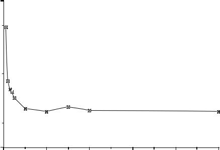
Figure 27: Near-asymptotic performance of distal supervised learning.

composite learning system. Because the actual plant output (y[n]) can still be measured after a learning trial, the true performance error (y [n] , y[n]) is still available for training the controller.13 This implies that the output of the forward model can be discarded; the forward model is needed only for the structure that it provides as part of the composite learning system (see below for further clari cation of this point). Moreover, for the purpose of providing internal structure to the learning algorithm, an exact forward model is not required. Roughly speaking, the forward model need only provide coarse information about how to improve the control signal based on the current performance error, not precise information about how to make the optimal correction. If the performance error is decreased to zero, then an accurate controller has been found, regardless of the path taken to nd that controller. Thus an accurate controller can be learned even if the forward model is inac-

13 This argument assumes that the subject actually performs the action. It is also possible to consider \mental practice" trials, in which the action is imagined but not performed (Minas, 1978). Learning through mental practice can occur by using the predicted performance error. This makes the empirically-testable prediction that the e cacity of mental practice should be closely tied to the accuracy of the underlying forward model (which can be assessed independently by measuring the subject's abilities at prediction or anticipation of errors).

53

Figure 28: Number of trials required to train the controller to an error criterion of 0.001 as a function of the number of trials allocated to training the forward model.

curate. This point is illustrated in Figure 28, which shows the time required to train an accurate controller as a function of the time allocated to training the forward model. The accuracy of the forward model increases monotonically as a function of training time, but is still somewhat inaccurate after 5000 trials (Jordan & Rumelhart, 1992). Note that the time required to train the controller is rather insensitive to the accuracy of the forward model.

Example

Further insight into the distal supervised learning approach can be obtained by reconsidering the linear problem described earlier. The composite learning system for this problem is shown in Figure 29. Note that we have assumed a perfect forward model|the parameters .5 and .4 in the forward model are those that describe the true plant. How might the performance error (y [n] , y[n]) be used to adjust the parameters v1 and v2 in the controller?

54

^

x [n]

D

Figure 29: The composite learning system (the controller and the forward model) for the rst-order example. The coe cients v1 and v2 are the unknown parameters in the controller. The coe cients :4 and :5 are the parameters in the forward model.

Suppose that the performance error is positive; that is, suppose that y [n] is greater than y[n]. Because of the positive coe cient (.4) that links u[n , 1] and y[n], to increase y[n] it su ces to increase u[n , 1]. To increase u[n , 1] it is necessary to adjust v1 and v2 appropriately. In particular, v1 should increase if x^[n , 1] is positive and decrease otherwise; similarly, v2 should increase if y [n] is positive and decrease otherwise. This algorithm can be summarized in an LMS-type update rule:

vi = sgn(w2) (y [n] , y[n])zi[n , 1];

where z1[n , 1] x^[n , 1], z2[n , 1] y [n], and sgn(w2) denotes the sign of w2 (negative or positive), where w2 is the forward model's estimate of the coe cient linking u[n , 1] and y[n] (cf. Equation 43).

Note the role of the forward model in this learning process. The forward model is required in order to provide the sign of the parameter w2 (the coe - cient linking u[n , 1] and y^[n]). The parameter w1 (that linking x^[n , 1] and y^[n]) is needed only during the learning of the forward model to ensure that the correct sign is obtained for w2. A very inaccurate forward model su ces for learning the controller|only the sign of w2 needs to be correct. Moreover, it is likely that the forward model and the controller can be learned simultaneously, because the appropriate sign for w2 will probably be discovered early in the learning process.

55

Reference Models

Throughout this chapter we have characterized controllers as systems that invert the plant dynamics. For example, a predictive controller was characterized as an inverse model of the plant|a system that maps desired plant outputs into the corresponding plant inputs. This mathematical ideal, however, is not necessarily realizable in all situations. One common di culty arises from the presence of constraints on the magnitudes of the control signals. An ideal inverse model moves the plant to an arbitrary state in a small number of time steps, the number of steps depending on the order of the plant. If the current state and the desired state are far apart, an inverse model may require large control signals, signals that the physical actuators may not be able to provide. Moreover, in the case of feedback control, large control signals correspond to high gains, which may compromise closed-loop stability. A second di culty is that the inverses of certain dynamical systems, known as \nonminimum phase" systems, are unstable (Astrom & Wittenmark, 1984). Implementing an unstable inverse model is clearly impratical, thus another form of predictive control must be sought for such systems.14

As these considerations suggest, realistic control systems generally embody a compromise between a variety of constraints, including performance, stability, bounds on control magnitudes, and robustness to disturbances. One way to quantify such compromises is through the use of a reference model. A reference model is an explicit speci cation of the desired input-output behavior of the control system. A simple version of this idea was present in the previous section when we noted that an inverse model can be de ned implicitly as any system that can be cascaded with the plant to yield the identity transformation. From the current perspective, the identity transformation is the simplest and most stringent reference model. An identity reference model requires, for example, that the control system respond to a sudden increment in the controller input with a sudden increment in the plant output. A more forgiving reference model would allow the plant output to rise more smoothly to the desired value. Allowing smoother changes in the plant output allows the control signals to be of smaller magnitude.

Although reference models can be speci ed in a number of ways, for example as a table of input-output pairs, the most common approach is to specify

14 A discussion of nonminimum phase dynamics is beyond the scope of this chapter, but an example would perhaps be useful. The system y[n + 1] = :5y[n] + :4u[n] , :5u[n , 1] is a nonminimum phase system. Solving for u[n] yields the inverse model u[n] = ,1:25y[n] + 2:5y [n + 1] + 1:25u[n , 1], which is an unstable dynamical system, due to the coe cient of 1:25 that links successive values of u.

56

the reference model as a dynamical system. The input to the reference model is the reference signal, which we now denote as r[n], to distinguish it from the reference model output, which we denote as y [n]. The reference signal is also the controller input. This distinction between the reference signal and the desired plant output is a useful one. In a model of speech production, for example, it might be desirable to treat the controller input as a linguistic \intention" to produce a given phoneme. The phoneme may be speci ed in a symbolic linguistic code that has no intrinsic articulatory or acoustic interpretation. The linguistic intention r[n] would be tied to its articulatory realization u[n] through the controller and also tied to its (desired) acoustic realization y [n] through the reference model. (The actual acoustic realization y[n] would of course be tied to the articulatory realization u[n] through the plant.)

Example

Let us design a model-reference controller for the rst-order plant discussed earlier. We use the following reference model:

where r[n] is the reference signal. This reference model is a second-order di erence equation in which the constant coe cients s1 and s2 are chosen to give a desired dynamical response to particular kinds of inputs. For example, s1 and s2 might be determined by specifying a particular desired response to a step input in the reference signal. Let us write the plant dynamical equation at time n + 2:

y[n + 2] = :5y[n + 1] + :4u[n + 1]:

We match up the terms on the right-hand sides of both equations and obtain the following control law:

Figure 30 shows the resulting model-reference control system. This control system responds to reference signals (r[n]) in exactly the same way as the reference model in Equation 45.

Note that the reference model itself does not appear explicitly in Figure 30. This is commonly the case in model-reference control; the reference model often exists only in the mind of the person designing or analyzing the control system. It serves as a guide for obtaining the controller, but it is not implemented as such as part of the control system. On the other hand, it is

57

Figure 30: The model-reference control system for the rst-order example.

also possible to design model-reference control systems in which the reference model does appear explicitly in the control system. The procedure is as follows. Suppose that an inverse model for a plant has already been designed. We know that a cascade of the inverse model and the plant yields the identity transformation. Thus a cascade of the reference model, the inverse model, and the plant yields a composite system that is itself equivalent to the reference model. The controller in this system is the cascade of the reference model and the inverse model. At rst glance this approach would appear to yield little net gain because it involves implementing an inverse model. Note, however, that despite the presence of the inverse model, this approach provides a solution to the problem of excessively large control signals. Because the inverse model lies after the reference model in the control chain, its input is smoother than the reference model input, thus it will not be required to generate large control signals.

Turning now to the use of reference models in learning systems, it should be clear that the distal supervised learning approach can be combined with the use of reference models. In the section on distal supervised learning, we described how an inverse plant model could be learned by using the identity transformation as a reference model for the controller and the forward model. Clearly, the identity transformation can be replaced by any other reference model and the same approach can be used. The reference model can be thought of as a source of input-output pairs for training the controller and the forward model (the composite learning system), much as the plant is a source of input-

58

output pairs for the training of the forward model. The distal supervised learning training procedure nds a controller that can be cascaded with the plant such that the resulting composite control system behaves as speci ed by the reference model.

It is important to distinguish clearly between forward and inverse models on the one hand and reference models on the other. Forward models and inverse models are internal models of the plant. They model the relationship between plant inputs and plant outputs. A reference model, on the other hand, is a speci cation of the desired behavior of the control system, from the controller input to the plant output. The signal that intervenes between the controller and the plant (the plant input) plays no role in a reference model speci cation. Indeed, the same reference model may be appropriate for plants having di erent numbers of control inputs or di erent numbers of states. A second important di erence is that forward models and inverse models are actual dynamical systems, implemented as internal models \inside" the organism. A reference model need not be implemented as an actual dynamical system; it may serve only as a guide for the design or the analysis of a control system. Alternatively, the reference model may be an actual dynamical system, but it may be \outside" of the organism and known only by its inputs and outputs. For example, the problem of learning by imitation can be treated as the problem of learning from an external reference model. The reference model provides only the desired behavior; it does not provide the control signals needed to perform the desired behavior.

Conclusions

If there is any theme that unites the various techniques that we have discussed, it is the important role of internal dynamical models in control systems. The two varieties of internal models|inverse models and forward models|play complementary roles in the implementation of sophisticated control strategies. Inverse models are the basic module for predictive control, allowing the system to precompute an appropriate control signal based on a desired plant output. Forward models have several roles: they provide an alternative implementation of feedforward controllers, they can be used to anticipate and cancel delayed feedback, they are the basic building block in dynamical state estimation, and they play an essential role in indirect approaches to motor learning. In general, internal models provide capabilities for prediction, control, and error correction that allow the system to cope with di cult nonlinear control problems.

It is important to emphasize that an internal model is not necessarily a

59

detailed model, or even an accurate model, of the dynamics of the controlled system. In many cases, approximate knowledge of the plant dynamics can be used to move a system in the \right direction." An inaccurate inverse model can provide an initial push that is corrected by a feedback controller. An inaccurate forward model can be used to learn an accurate controller. Inaccurate forward models can also be used to provide partial cancellation of delayed feedback, and to provide rough estimates of the state of the plant. The general rule is that partial knowledge is better than no knowledge, if used appropriately.

These observations would seem to be particularly relevant to human motor control. The wide variety of external dynamical systems with which humans interact, the constraints on the control system due to delays and limitations on force and torque generation, and the time-varying nature of the musculoskeletal plant all suggest an important role for internal models in biological motor control. Moreover, the complexity of the systems involved, as well as the unobservability of certain aspects of the environmental dynamics, make it likely that the motor control system must make do with approximations. It is of great interest to characterize the nature of such approximations. Although approximate internal models can often be used e ectively, there are deep theoretical issues involved in characterizing how much inaccuracy can be tolerated in various control system components. The literature on control theory is replete with examples in which inaccuracies lead to instabilities, if care is not taken in the control system design. As theories of biological motor control increase in sophistication, these issues will be of increasing relevance.

References

Anderson, B. D. O., & Moore, J. B. (1979). Optimal Filtering. Englewood Cli s, NJ: Prentice-Hall.

Astrom, K. J., & Wittenmark, B. (1984). Computer controlled systems: Theory and design. Englewood Cli s, NJ: Prentice-Hall.

Astrom, K. J., & Wittenmark, B. (1989). Adaptive Control. Reading, MA: Addison-Wesley.

Atkeson, C. G., & Reinkensmeyer, D. J. (1988). Using associative contentaddressable memories to control robots. IEEE Conference on Decision and Control. San Francisco, CA.

60