

funct_r_z
.pdfAlgorithm
See also
The relax function returns a square matrix in which:
•an element's location in the matrix corresponds to its location within the square region, and
•its value approximates the value of the solution at that point.
This function uses the relaxation method to converge to the solution. Poisson's equation on a square domain is represented by:
aj, kuj + 1, k + bj, kuj – 1, k + cj, kuj, k + 1 + dj, kuj, k – 1 + ej, kuj, k = fj, k .
Gauss-Seidel with successive overrelaxation (Press et al., 1992)
multigrid
reverse |
Sorting |
One-dimensional Case
Syntax reverse(v)
Description Reverses the order of the elements of vector v.
Arguments
v vector
Two-dimensional Case
Syntax |
reverse(A) |
Description |
Reverses the order of the rows of matrix A. |
Arguments |
|
A |
matrix |
See also |
See sort for sample application. |
rexp
Syntax
Description
Arguments
m
r
See also
Algorithm
Random Numbers
rexp(m, r)
Returns a vector of m random numbers having the exponential distribution.
integer, m > 0 real rate, r > 0
rnd
Inverse cumulative density method (Press et al., 1992)
Functions |
97 |

rF |
Random Numbers |
Syntax |
rF(m, d1, d2) |
Description |
Returns a vector of m random numbers having the F distribution. |
Arguments |
integer, m > 0 |
m |
|
d1, d2 |
integer degrees of freedom, d1 > 0, d2 > 0 |
Algorithm |
Best’s XG algorithm, Johnk’s generator (Devroye, 1986) |
See also |
rnd |
rgamma |
Random Numbers |
Syntax |
rgamma(m, s) |
Description |
Returns a vector of m random numbers having the gamma distribution. |
Arguments |
integer, m > 0 |
m |
|
s |
real shape parameter, s > 0 |
Algorithm |
Best’s XG algorithm, Johnk’s generator (Devroye, 1986) |
See also |
rnd |
rgeom |
Random Numbers |
Syntax |
rgeom(m, p) |
Description |
Returns a vector of m random numbers having the geometric distribution. |
Arguments |
integer, m > 0 |
m |
|
p |
real number, 0 < p ≤ 1 |
Algorithm |
Inverse cumulative density method (Press et al., 1992) |
See also |
rnd |
98 |
Chapter 1 Functions |

rhypergeom
Syntax
Description
Arguments
m
a, b, n
Algorithm
See also
Random Numbers
rhypergeom(m, a, b, n)
Returns a vector of m random numbers having the hypergeometric distribution.
integer, m > 0
integers, 0 ≤ a , 0 ≤ b , 0 ≤ n ≤ a + b
Uniform sampling methods (Devroye, 1986)
rnd
rkadapt |
(Professional) |
Differential Equation Solving |
Syntax |
rkadapt(y, x1, x2, acc, D, kmax, save) |
|
Description |
Solves a differential equation using a slowly varying Runge-Kutta method. Provides DE solution |
|
|
estimate at x2. |
|
Arguments |
Several arguments for this function are the same as described for rkfixed. |
|
y |
real vector of initial values |
|
x1, x2 |
real endpoints of the solution interval |
|
D(x, y) |
real vector-valued function containing the derivatives of the unknown functions |
|
acc |
real acc > 0 controls the accuracy of the solution; a small value of acc forces the algorithm to |
|
|
take smaller steps along the trajectory, thereby increasing the accuracy of the solution. Values |
|
|
of acc around 0.001 will generally yield accurate solutions. |
|
kmax |
integer kmax > 0 specifies the maximum number of intermediate points at which the solution |
|
|
will be approximated. The value of kmax places an upper bound on the number of rows of the |
|
|
matrix returned by these functions. |
|
save |
real save > 0 specifies the smallest allowable spacing between the values at which the solutions |
|
|
are to be approximated. save places a lower bound on the difference between any two numbers |
|
|
in the first column of the matrix returned by the function. |
|
Comments
Algorithm
See also
The specialized DE solvers Bulstoer, Rkadapt, Stiffb, and Stiffr provide the solution y(x) over a number of uniformly spaced x-values in the integration interval bounded by x1 and x2. When you want the value of the solution at only the endpoint, y(x2), use bulstoer, rkadapt, stiffb, and stiffr instead.
Adaptive step 5th order Runge-Kutta method (Press et al., 1992)
rkfixed, a more general differential equation solver, for information on output and arguments;
Rkadapt.
Functions |
99 |

Rkadapt |
(Professional) |
Differential Equation Solving |
Syntax |
Rkadapt(y, x1, x2, npts, D) |
|
Description |
Solves a differential equation using a slowly varying Runge-Kutta method; provides DE solution |
|
|
at equally spaced x values by repeated calls to rkadapt. |
|
Arguments |
All arguments for this function are the same as described for rkfixed. |
|
y |
real vector of initial values |
|
x1, x2 |
real endpoints of the solution interval |
|
npts |
integer npts > 0 specifies the number of points beyond initial point at which the solution is to be |
|
|
approximated; controls the number of rows in the matrix output |
|
D(x, y) |
real vector-valued function containing the derivatives of the unknown functions |
|
Comments |
Given a fixed number of points, you can approximate a function more accurately if you evaluate |
|
|
it frequently wherever it's changing fast, and infrequently wherever it's changing more slowly. |
|
|
If you know that the solution has this property, you may be better off using Rkadapt. Unlike |
|
|
rkfixed which evaluates a solution at equally spaced intervals, Rkadapt examines how fast the |
|
|
solution is changing and adapts its step size accordingly. This “adaptive step size control” enables |
|
|
Rkadapt to focus on those parts of the integration domain where the function is rapidly changing |
|
|
rather than wasting time on the parts where change is minimal. |
|
|
Although Rkadapt will use nonuniform step sizes internally when it solves the differential |
|
|
equation, it will nevertheless return the solution at equally spaced points. |
|
|
Rkadapt takes the same arguments as rkfixed, and the matrix returned by Rkadapt is identical |
|
|
in form to that returned by rkfixed. |
|
Algorithm |
Fixed step Runge-Kutta method with adaptive intermediate steps (5th order) (Press et al., 1992) |
|
See also |
rkfixed, a more general differential equation solver, for information on output and arguments. |
|
|
|
|
rkfixed |
|
Differential Equation Solving |
Syntax |
rkfixed(y, x1, x2, npts, D) |
|
Description |
Solves a differential equation using a standard Runge-Kutta method. Provides DE solution at |
|
|
equally spaced x values. |
|
Arguments
yreal vector of initial values (whose length depends on the order of the DE or the size of the system
of DEs). For a first order DE like that in Example 1 or Example 2 below, the vector degenerates to one point, y(0) = y(x1) . For a second order DE like that in Example 3, the vector has two
elements: the value of the function and its first derivative at x1. For higher order DEs like that in Example 4, the vector has n elements for specifying initial conditions of y, y¢, y², ¼, y(n – 1) .
For a first order system like that in Example 5, the vector contains initial values for each unknown function. For higher order systems like that in Example 6, the vector contains initial values for the n – 1 derivatives of each unknown function in addition to initial values for the functions themselves.
x1, x2 real endpoints of the interval on which the solution to the DEs will be evaluated; initial values in y are the values at x1.
100 |
Chapter 1 Functions |

npts integer npts > 0 specifies the number of points beyond the initial point at which the solution is to be approximated; controls the number of rows in the matrix output.
D(x, y) |
real vector-valued function containing derivatives of the unknown functions. For a first order DE |
||||
|
like that in Example 1 or Example 2, the vector degenerates to a scalar function. For a second |
||||
|
order DE like that in Example 3, the vector has two elements: |
|
|
||
|
|
|
|
y¢(t) |
|
|
D(t, y) = |
y¢(t) |
|
|
|
|
|
y²(t) |
|
||
|
y²(t) |
|
|
||
|
|
|
|
||
|
|
|
. |
|
|
|
|
|
|
|
|
|
For higher order DEs like that in Example 4, the vector has n elements: D(t, y) = |
. |
|||
|
. |
||||
|
|
|
|
|
|
|
|
|
|
. |
|
|
|
|
|
y(n)(t ) |
|
|
|
|
|
|
|
For a first order system like that in Example 5, the vector contains the first derivatives of each unknown function. For higher order systems like that in Example 6, the vector contains expressions for the n – 1 derivatives of each unknown function in addition to nth derivatives.
Examples
Example 1: Solving a first order differential equation.
Functions |
101 |

Example 2: Solving a nonlinear differential equation.
Example 3: Solving a second order differential equation.
102 |
Chapter 1 Functions |

.
Example 4: Solving a higher order differential equation.
Example 5: Solving a system of first order linear equations.
Functions |
103 |
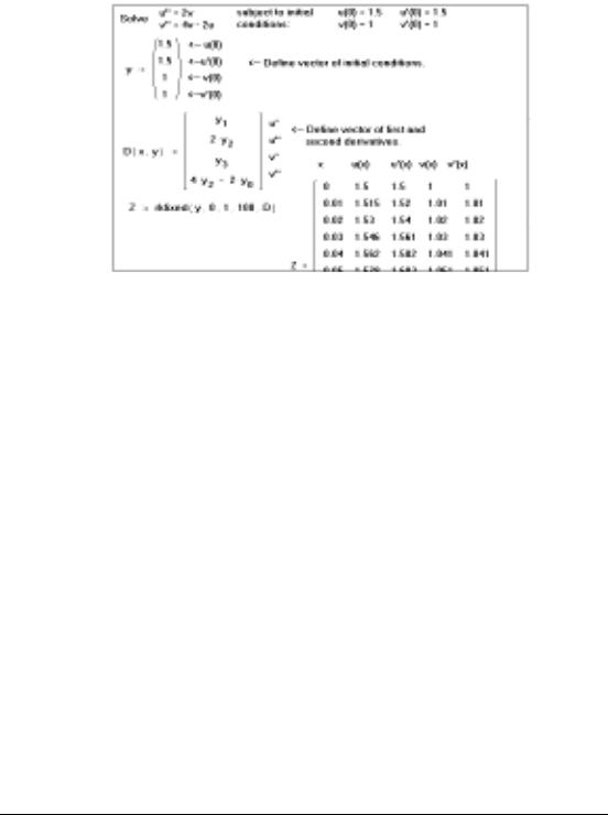
Example 6: Solving a system of second order linear differential equations.
Comments For a first order DE like that in Example 1 or Example 2, the output of rkfixed is a two-column matrix in which:
•The left-hand column contains the points at which the solution to the DE is evaluated.
•The right-hand column contains the corresponding values of the solution.
For a second order DE like that in Example 3, the output matrix contains three columns: the lefthand column contains the t values; the middle column contains y(t) ; and the right-hand column contains y′(t) .
For higher order DEs like that in Example 4, the output matrix contains n columns: the left-hand one for the t values and the remaining columns for values of y(t), y¢(t), y²(t), ¼, y(n – 1)(t) .
For a first order system like that in Example 5, the first column of the output matrix contains the points at which the solutions are evaluated and the remaining columns contain corresponding values of the solutions. For higher order systems like that in Example 6:
•The first column contains the values at which the solutions and their derivatives are evaluated.
•The remaining columns contain corresponding values of the solutions and their derivatives. The order in which the solutions and their derivatives appear matches the order in which you put them into the vector of initial conditions.
The most difficult part of solving a DE is defining the function D(x, y). In Example 1 and Example 2, for example, it was easy to solve for y¢(x ) . In some more difficult cases, you can solve for y¢(x) symbolically and paste it into the definition for D(x, y). To do so, use the solve keyword or the Solve for Variable command from the Symbolics menu.
The function rkfixed uses a fourth order Runge-Kutta method, which is a good general-purpose DE solver. Although it is not always the fastest method, the Runge-Kutta method nearly always succeeds. There are certain cases in which you may want to use one of Mathcad's more specialized DE solvers. These cases fall into three broad categories:
104 |
Chapter 1 Functions |

Algorithm
See also
•Your system of DEs may have certain properties which are best exploited by functions other than rkfixed. The system may be stiff (Stiffb, Stiffr); the functions could be smooth (Bulstoer) or slowly varying (Rkadapt).
•You may have a boundary value rather than an initial value problem ( sbval and bvalfit).
•You may be interested in evaluating the solution only at one point ( bulstoer, rkadapt, stiffb and stiffr).
You may also want to try several methods on the same DE to see which one works the best. Sometimes there are subtle differences between DEs that make one method better than another.
Fixed step 4th order Runge-Kutta method (Press et al., 1992)
Mathcad Resource Center QuickSheets and Differential Equations tutorial.
rlnorm |
Random Numbers |
Syntax |
rlnorm(m, μ, σ) |
Description |
Returns a vector of m random numbers having the lognormal distribution. |
Arguments |
integer, m > 0 |
m |
|
μ |
real logmean |
σ |
real logdeviation, σ > 0 |
Algorithm |
Ratio-of-uniforms method (Devroye, 1986) |
See also |
rnd |
|
|
rlogis |
Random Numbers |
Syntax |
rlogis(m, l, s) |
Description |
Returns a vector of m random numbers having the logistic distribution. |
Arguments |
integer, m > 0 |
m |
|
l |
real location parameter |
s |
real scale parameter, s > 0 |
Algorithm |
Inverse cumulative density method (Press et al., 1992) |
See also |
rnd |
Functions |
105 |

rnbinom
Syntax
Description
Arguments
m, n
p
Algorithm
See also
Random Numbers
rnbinom(m, n, p)
Returns a vector of m random numbers having the negative binomial distribution.
integers, m > 0, n> 0 real number, 0 < p ≤ 1
Based on rpois and rgamma (Devroye, 1986)
rnd
rnd |
Random Numbers |
Syntax rnd(x)
Description Returns a random number between 0 and x. Identical to runif(1, 0, x) if x > 0 .
Arguments
x real number
Example
Note: You won’t be able to recreate this example exactly because the random number generator gives different numbers every time.
Comments Each time you recalculate an equation containing rnd or some other random variate built-in function, Mathcad generates new random numbers. Recalculation is performed by clicking on the equation and choosing Calculate from the Math menu.
106 |
Chapter 1 Functions |