

Design of an active acoustic sensor system for an autonomous underwater vehicle
.pdfChapter 6 Hardware Verification and Experimental Results
This result is the same as the time measured from the oscilloscope in Figure 6.2.
It is therefore verified that the TPU channels can be triggered by a falling signal edge and the digital output is functioning correctly. The echo sounder should therefore interface properly with the Eyebot. This also demonstrates the accuracy of the TPU channels at detecting the edges.
6.1.2 Testing the Echo Sounder Interface
The echo sounder interface also needs to be tested to ensure that the correct voltages and signals are received and transmitted, before connection to the Eyebot. The experimental set up involves connecting the echo sounder’s key input to the digital output of the Eyebot, through a 1kΩ resistor. The logic output of the echo sounder is then measured using an oscilloscope to analyse the signal and the voltage output.
The experiment is to determine if the signal at the logic output is compatible with the TPU and to see if the digital output is compatible with the key input.
The test code is just the transmission of the 200µs pulse from the digital output to the key input of the echo sounder.
Figure 6.3 demonstrates the experimental set up.
Figure 6.3: The experimental setup for the echo sounder interface
Figure 6.4 shows the signal when no pulse is sent from the Eyebot.
47
Design of an Active Acoustic Sensor System
Figure 6.4: No signal through the echo sounder
What is learnt from Figure 6.4 is that there is a 12.19V signal that is transmitted through the logic output of the echo sounder. The reason for this is that the signal does not have a reference. This is unacceptable because the TPU channels can only accept a voltage of 5V at its pin. To solve this problem, a pull down resistor needs to be used. This is to be placed between the logic output and the ground of the echo sounder. This properly grounds the signal and converts it to one that is compatible with the TPU channel.
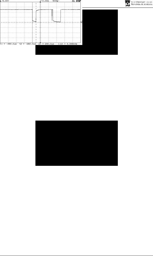
Figure 6.5: 200µs pulse sent via the digital output, and the transducer is placed in water
Figure 6.5 demonstrates the presence of echoes that are returned to the echo sounder, as conjectured during the design stage of the echo sounder. These need to be handled by the TPU channel. The setting of the MAX_COUNT parameter for the TPU as stated in section 5.3.2 should result in only one echo registering with the TPU. The proper reception of pulses indicates that the digital output is at a sufficient voltage to key the echo sounder circuit.
The echo sounder has been modified according to the tests performed on the echo sounder interface. In Figure 6.6, a 10kΩ trimpot resistor is used as a pull down resistor. Figure 6.7 shows that the voltage of the logic output of the echo sounder has changed to 4.63V due to the resistor. This makes it compatible with the TPU channel.
48

Chapter 6 Hardware Verification and Experimental Results
Figure 6.6: the pull down resistor placed between the logic output and the ground
Figure 6.7: Signal when pull down resistor is used
6.1.3 Testing the Combined Interface
The experimental set up for the combined interface is exactly the same as the one used for the echo sounder interface, except that the logic output of the echo sounder is now connected to the TPU channels.
Figure 6.8: The experimental setup for the combined interface
49
Design of an Active Acoustic Sensor System
An experiment is conducted to verify that the echo sounder and the Eyebot are correctly interfaced together.
The test code implemented for this experiment starts the TPU channel and then transmits a 200µs pulse. A key deactivated wait then precedes a display of the time of flight for the signal on the Eyebot LCD screen.
To test for the functionality of the echo sounder interface, two experiments test for the two cases which the echo sounder should detect.
The first case is when the echo sounder does not receive any returned pulse. This is simulated by removing the transducer from the water.
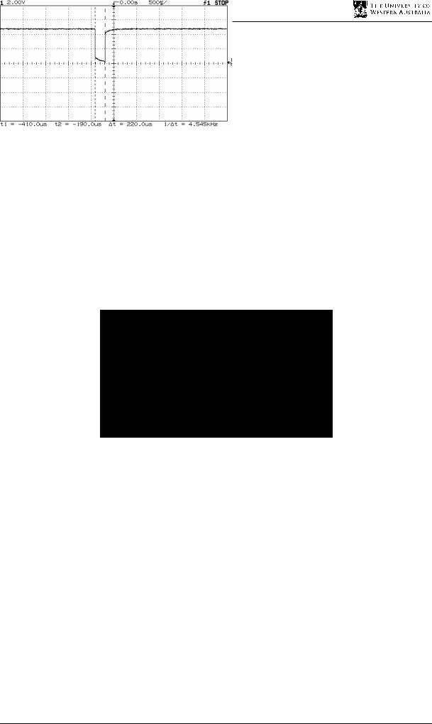
The test verified, as in figure 6.9, that the TPU channel does not receive a second falling edge meaning that the CPU is not interrupted. A time out needs to be called for this situation and a maximum time difference recorded by the Eyebot to signify that a real value cannot be calculated because the surface is either out of range or the transducer is not in the water.
Figure 6.9: Signal at the TPU channel when the transducer is not in the water
The second experiment is to represent a successful transmission of the signal. This is accomplished by placing the echo sounder in a small container of water. This will result in significant reverberation, or echoing, which tests to see if the echo sounder can account for this and only detect the first echo (the first falling edge on the logic output from the echo sounder).
50
Chapter 6 Hardware Verification and Experimental Results
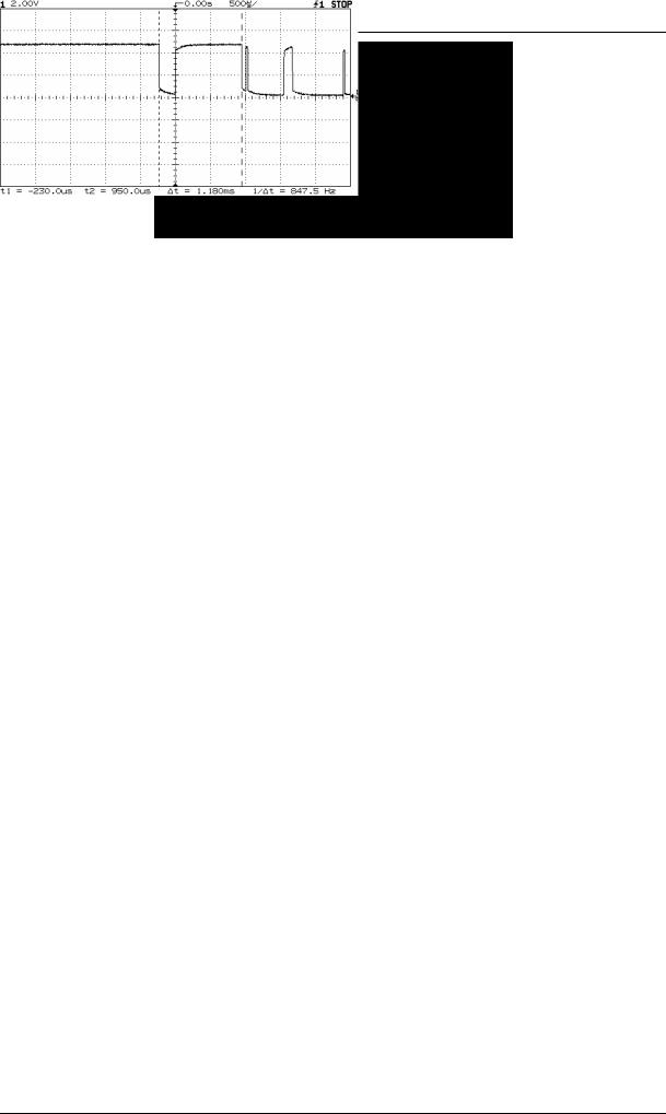
Figure 6.10: Signal that is received at the TPU channel when the transducer is in the water
Figure 6.10 shows the signal transmitted to the Eyebot from the logic output of the echo sounder. Notice the multiple secondary echoes that the TPU channel must handle. The measured time difference from the oscilloscope is compared with the actual time difference recorded by the Eyebot and displayed on the LCD screen. The time difference as measured using the oscilloscope is 1.180ms. The time difference recorded by the Eyebot is 4945 counts. Now each count represents a time of 238.4ns since the smallest resolution is being used (refer to Appendix B), so the actual time is:
time =Tc1 ×number of counts = 238.4(10−9 )×4945
time =1.179×10⁻³ sec
This is approximately the same value as the value attained by measuring the time on the oscilloscope.
The interface can be seen to be functioning according to the specification required. The signals have been properly matched to suit the voltage requirements of the TPU channels. The transmitted and received pulses are correctly identified by the TPU channels and the time of flight can be properly calculated. Thus the interface has been verified to function correctly.
6.2 Determining the Characteristics of Echo Sounding
Once the interface between the Eyebot and the echo sounder is established, it is necessary to determine the exact physical characteristics of the echo sounder sensor. For these experiments, the timing out of the channel is not necessary and thus has not been included in the code set for testing.
51

Design of an Active Acoustic Sensor System
6.2.1 The Linearity of Returns
To verify that the C functions programmed for the echo sounder allowed the Eyebot to determine the time of flight of the signal, the echo sounder was tested in a long channel of water in the Hydraulics Laboratory within the university.
The interface was connected, as outlined in Section 6.1.3. To ensure that that there is a constant voltage supply to both the Eyebot and the echo sounder, both power supplies are voltage regulated power supplies.
The test script for the Eyebot to test the echo sounder is as follows:
•Initialise the required TPU channel
Then cycle through a loop consisting of the following:
•Start the TPU channel
•Transmit a 200µs pulse from the Eyebot
•Wait until a key is pressed to ensure that an interrupt has occurred
•Display the time of flight on the LCD screen
The loop is to obtain different values for the same location. The results are collected over a distance from 0.18m to 3.5m and then the values for each distance point is then averaged to give an average time of flight for the distance point.
|
|
Time of Flight for Signal vs distance |
|
||
|
20000 |
|
|
|
|
|
18000 |
|
|
|
|
(counts) |
16000 |
|
|
|
|
14000 |
|
|
|
|
|
12000 |
|
|
|
|
|
flight |
10000 |
|
|
|
|
8000 |
|
|
|
|
|
of |
|
|
|
|
|
|
|
|
|
|
|
Time |
6000 |
|
|
|
|
4000 |
|
|
|
|
|
|
|
|
|
|
|
|
2000 |
|
|
|
|
|
0 |
|
|
|
|
|
0 |
1 |
2 |
3 |
4 |
|
|
|
Distance to wall (m) |
|
|
Figure 6.11: Calculated time of flight over a range of distances for the echo sounder
52

Chapter 6 Hardware Verification and Experimental Results
Figure 6.11 is a plot of the experiment, which demonstrates a linear relationship between the time of flight and the distance to the surface. A statistical analysis of the data shows that gradient of the function is 5.653x10³ counts/metre.
6.2.2 Calibrating the Echo Sounder
For different types of water and for different temperatures, the speed of sound will vary. It is vital for the accuracy of the echo sounder that the system be correctly calibrated for the type of environment in which it will be used.
Given a set of data, like the set in Figure 6.11, it is possible to obtain the speed of sound in the test medium. Now each data point represents a particular time of flight for a given distance. Assuming that all the data is linear, then the change in time per unit distance between any two points equates to the instantaneous rate of change of time with respect to distance.
dt |
= |
∆t |
(6.1) |
|
ds |
∆s |
|||
|
|
When this gradient is inverted, it becomes a rate of change of distance with respect to time. This is the speed of sound in the medium.
cm |
= |
ds |
(6.2) |
|
dt |
||||
|
|
|
So by finding the gradient for the line of regression of the data points, it is possible to determine the speed of sound in the medium. Not only is this result useful for calibrating the echo sounder, but it also has applications where the speed characteristic of a particular environment is required.
To test this theory, the data set in Figure 6.11 is used. The line of regression for the data has a gradient of:
dtc |
= 5.653×10 |
3 |
counts / metre |
(6.3) |
dsw |
|
|
where tc is the time in counts and sw is the distance to the surface.
This value must be halved to account for the fact that the sound wave must travel the distance twice, once away from the echo sounder and once returning to the echo sounder.
53

Design of an Active Acoustic Sensor System
dtc = 2.826×10³ counts / metre dsr
where sr represents the round trip distance.
Converting the counts to time in seconds using the set resolution of 238.4ns results in the following:
|
dt |
= 2.826(103 )×238.4(10−9 ) |
|
|||
|
dsr |
|
||||
|
|
|
|
|
|
|
|
dt |
= 6.738×10⁻⁴ sec/ metre |
|
|||
|
dsr |
|
||||
|
|
|
|
|
|
|
Inverting this result will give the speed of sound in the medium. |
|
|||||
|
|
cm = |
dsr |
|
|
(6.4) |
|
|
dt |
||||
|
|
|
||||
|
|
1 |
|
|
||
|
|
= |
|
|
|
|
|
|
6.738×10⁻⁴ |
|
|||
cm =1.484×10³ m / s
This result is closely approximates the speed of sound in fresh water, which is 1481m/s.
6.2.3 Mean Square Error for the Echo Sounder
Whilst the data appears to be linear, there is some error, even in the averaged data for the plot.
The root mean square (RMS) error for the data from the line of best fit is calculated to be 167.2 counts. The RMS error is calculated by subtracting the predicted value from the observed value to result in an error, which is then squared. The average of the squared values is taken to form the mean square value. The RMS value is just the square root of the mean square value.
The 167.2 counts RMS will result in an error of margin of:
distance error = count error ×resolution |
×speed of sound |
|
||||
|
2 |
|
|
|
|
|
= |
167.2×238.4(10−9 ) |
×1484 |
(6.5) |
|||
|
2 |
|
||||
|
|
|
|
|||
|
|
|
|
|
||
distance error = 2.96×10⁻² m
Assuming that the speed of sound in the water is 1484m/s as in equation 6.5.
54

Chapter 6 Hardware Verification and Experimental Results
The error is, in part, due to the difficulty in precisely measuring the distance from the transducer to the surface of the wall.
This error is significant but not large in comparison to the size of the AUV itself and the pool environment for which it will be competing in. As the minimum requirement for the resolution of the echo sounder is 5cm, as stated in chapter 3, this result means that the current echo sounder is sufficient for the resolution requirement.
This result will be important for the EKF equations that will be discussed in Chapter 7. The error covariance is required to complete the correction cycle of the EKF. If the error, or noise, is assumed to be additive white Gaussian noise (AWGN), then the covariance of this noise is the mean square value for the error. For this instance, the covariance is 8.76x10⁻⁴ m2.
This means that the measurement noise for the sensor will have a normal distribution of:
p(w)~ N (0,8.76 ×10−4 ) |
(6.6) |
The result is used by the EKF to better model the sensor readings, allowing for more accurate estimations of state, as will be discussed in Chapter 7.
This error covariance will not be the same for all environments and will need to be calculated for each environment.
6.2.4 Minimum Detectable Static Distance
What can also be noted from Figure 6.11 is that there is a minimum detectable distance for the echo sounder. This range can be observed to be approximately 0.25m. The theoretical value of this distance can be calculated from the time of the ringing in the transducer, which is 220µs, as in Figure 6.9:
min distance = min time×speed of sound 2
= 220(10−6 )×1484 (6.7) 2
min distance = 0.163m
There is a discrepancy between the measured data and the real data. This is due to the signal having to traverse the length of the transducer cable twice, resulting in a greater time between the pulses, and consequently a slightly greater minimum distance. Thus the minimum detectable static distance in fresh water is 0.163m.
55
Design of an Active Acoustic Sensor System
6.2.5 Maximum Detectable Static Distance
For active sonar, according to the formula given in Chapter 2, the detection threshold is the signal level at which the arriving signal can be detected 50% of the time.
The echo sounder is therefore tested to determine the distance that the device can no longer detect the arriving signal for 50% of the time. To test for the maximum range of the echo sounder, the same set up for determining the linearity of the sonar returns was employed.
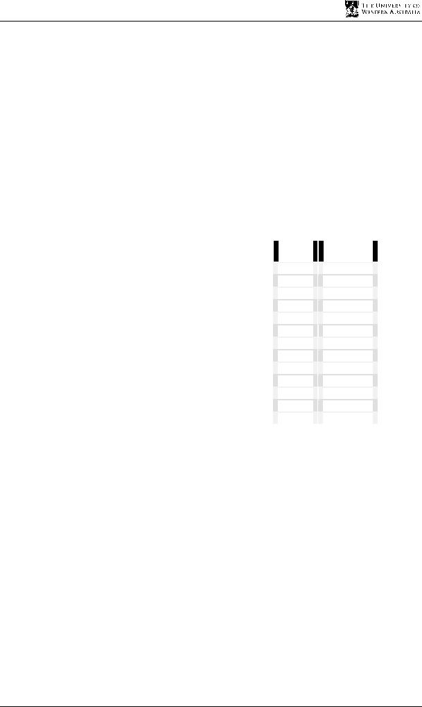
Starting at a distance of 2m from the surface of the reflecting wall, 500 measurements are taken to determine whether the signal has been detected for over 50% of the time. Table 6.1 shows the results of the experiment.
Distance |
Sample |
Sample |
Sample |
Sample |
|
Sample |
|
Detection |
|||||
(m) |
1 |
|
2 |
|
3 |
|
4 |
|
|
5 |
|
Percentage |
|
|
|
|
|
|
|
|
|
|
|
|
|
|
|
2 |
|
100 |
|
100 |
|
97 |
|
98 |
|
|
100 |
|
99 |
|
|
|
|
|
|
|
|
|
|
|
|
||
2.2 |
|
100 |
|
100 |
|
99 |
|
98 |
|
|
100 |
|
99.4 |
|
|
|
|
|
|
|
|
|
|
|
|
||
2.4 |
|
100 |
|
100 |
|
98 |
|
98 |
|
|
100 |
|
99.2 |
|
|
|
|
|
|
|
|
|
|
|
|
||
2.6 |
|
99 |
|
100 |
|
98 |
|
98 |
|
|
99 |
|
98.8 |
|
|
|
|
|
|
|
|
|
|
|
|
||
2.8 |
|
99 |
|
99 |
|
97 |
|
98 |
|
|
98 |
|
98.2 |
|
|
|
|
|
|
|
|
|
|
|
|
|
|
3 |
|
99 |
|
97 |
|
97 |
|
100 |
|
|
97 |
|
98 |
|
|
|
|
|
|
|
|
|
|
|
|
||
3.2 |
|
90 |
|
82 |
|
87 |
|
88 |
|
|
82 |
|
85.8 |
|
|
|
|
|
|
|
|
|
|
|
|
||
3.4 |
|
95 |
|
98 |
|
99 |
|
98 |
|
|
99 |
|
97.8 |
|
|
|
|
|
|
|
|
|
|
|
|
||
3.6 |
|
87 |
|
97 |
|
90 |
|
89 |
|
|
88 |
|
90.2 |
|
|
|
|
|
|
|
|
|
|
|
|
||
3.8 |
|
13 |
|
18 |
|
18 |
|
14 |
|
|
14 |
|
15.4 |
|
|
|
|
|
|
|
|
|
|
|
|
|
|
4 |
|
14 |
|
19 |
|
14 |
|
19 |
|
|
15 |
|
16.2 |
|
|
|
|
|
|
|
|
|
|
|
|
||
4.2 |
|
1 |
|
2 |
|
1 |
|
1 |
|
|
2 |
|
1.4 |
|
|
|
|
|
|
|
|
|
|
|
|
||
4.4 |
|
0 |
|
0 |
|
0 |
|
0 |
|
|
0 |
|
0 |
Table 6.1: Samples for sonar returns for distances from 2.4m to 3.5m
Table 6.1 shows that the detection of the return signal begins to significantly drop at 3.8m. At distances longer than 3.8m, the detection begins to drop to 0% making it extremely difficult for the AUV to detect obstacles.
Figure 6.12 shows the result of Table 6.1 in a graphical form.
The reason for the increasing lack of detection after 3.8m is that the signal becomes attenuated to a level that is undetectable by the echo sounder. Thus the maximum detectable static distance is 3.8m in fresh water.
56