Bonissone P.P.Fuzzy logic and soft computing.Technology development and applications

16.1.2Solution Description

System Architecture The overall scheme for the proposed train handling is shown in Figure 22. It consists of an FPI closing the loop around the train simulation (TSIM), using only the current velocity as its state input. This speed and lookahead are compared with the desired pro le to generate a predicted near-term error as input to the FPI, which outputs control actions back to the simulator. O ine, a GA uses the setup for evaluating various FPI parameters.

Figure 22: System schematic for using a GA to tune a fuzzy train controller.

The simulator | TSIM, is an in-house implementation, combining internal data with physical/empirical models as described in TEM (Train Energy Model) [Drish, 1992]. TEM was developed by the Association of American Railroads. TSIM simulates an extended train with arbitrary detailed makeup, over a speci ed track pro le. The version of TSIM used here does not simulate a stretchable train for the sake of computational e ciency.

For the purpose of this study, GENESIS (GENEtic Search Implementation System) has been adopted as a software development tool. It has been developed by John J. Grefenstette to promote the study of genetic algorithms for function optimization. The user must provide only a \ tness" function which returns a corresponding value for any point in the search space.

Fitness Functions To study the e ects of di erent objectives, we minimize three tness functions :

P jvi , vdj

+w2 i K2 i

vd denotes the desired velocity and i is a distance or milepost index. f1 captures throttle jockeying, f2 captures speed pro le tracking accuracy, and f3 combines a weighted sum of the two.

Tuning the Fuzzy PI

Testbed and Design Choices For comparison purposes, twelve tests have been conducted by taking a cross-product of: the scaling factor values before and after GA tuning, the membership function parameter

51

values before and after GA tuning, and the 3 tness functions. The tests are designed to demonstrate that GAs are powerful search methods and are very suitable for automated tuning of FPI controllers. GAs are able to come up with near-optimal FPI controllers within a reasonable amount of time according to di erent search criteria. In addition, the tests are also designed to demonstrate that we should tune parameters in the order of their signi cance. That is, we should tune scaling factors rst since they have global e ects on all the control rules in a rule base. Tuning membership functions will only give marginal improvements for a FPI with tuned scaling factors. In the following, we present testbed set-up and design choices in brief.

Train Simulator Parameters: All testing for the automated tuning of FPI was done using TSIM. Two track pro les were used: an approximately 14 mile at track and an approximately 40 mile piece of actual track from Selkirk to Framingham over the Berkshires. The train was nearly 9000 tons, and about a mile long, with 4 locomotives and 100 loaded railcars. An analytically computed velocity pro le which minimizes fuel consumption was used as the reference.

FPI Controller Parameters: The standard termset used in the FPI is fNH, NM, NL, ZE, PL, PM, PHg, where N = Negative, P = Positive, H = High, M = Medium, L = Low, and ZE = Zero. Initially, these seven terms are uniformly positioned trapezoids overlapping at a 50% level over the normalized universe of discourse. This is illustrated in Figure 23. Since the controller is de ned by a nonlinear control surface in

Initial MF for e, de, & du

initial

1.00

0.90

0.80

0.70

0.60

0.50

0.40

0.30

0.20

0.10

0.00

Figure 23: Fuzzy membership functions

(e; e; u) space, we need three termsets in all, one for each of e; e, u. The design leads to a symmetric controller, which is not always a good assumption. In this case, the GA tuning will automatically create the required asymmetry.

GENESIS parameters: The GA parameters are : Population Size = 50, Crossover Rate = 0.6, Mutation Rate = 0.001. In addition, all structures in each generation were evaluated, the elitist strategy was used to guarantee monotone convergence, gray codes were used in the encodings, and selection was rank based.

Tuning of Scaling Factors (SF): Each chromosome is represented as a concatenation of three 3-bit values for the three oating point values for the three FPI scaling factors Se , Sd and Su. They are in the

ranges: Se 2 [1; 9]; Sd 2 [0:1; 0:9]; Su 2 [1000; 9000]. The intent is to demonstrate a GA's ability for function optimization even with such a simple 9-bit chromosome.

Tuning of Membership Functions (MF): Each MF is trapezoidal and parameterized by left base (L), center base (C), and right base (R), as illustrated in Figure 24.

If we did not have any constraints on the membership functions (MFs), we would need 21 parameters to represent each termset. In our case we want to impose certain conditions on the MFs to enforce some good design rules. Since each MF is trapezoidal and we want to maintain an overlap of degree equal to 0.5 between adjacent trapezoids, this restriction partitions the universe of discourse into disjoint intervals, denoted by

bi, which alternate between being cores and the overlap areas of the MFs. Furthermore, the cores of NH and P H extend semi-in nitely to the left and right respectively (outside the [-1,1] interval). We also want

52

Figure 24: Membership function representation.

to maintain a symmetry between the core of NH and P H with respect to the mid point of the scale (0). Finally, the sum of all the disjoint intervals should be equal to 2. The above constraints translate into the following relations:

Li = Ri+1 for i = 1; . . .; 6 - [0.5 overlap]

R1 = L7 = 0 - [Extension outside the [-1,1] interval]

(b1 = C1) = (b13 = C7) - [Symmetry of extreme labels]

12

C1 = 2,P2i=2 bi - [interval normalization]

Therefore, in this case we need eleven intervals, denoted by bi, to represent the seven 7 MF labels in each termset. In general, under the above conditions, the number of required intervals j b j is:

j b j= (2 j MF j ,3)

where j MF j is the number of membership functions. Each termset is represented by a vector of 11 oating point values. For the present study, each bi is set within the range of [0:09; 0:18] and the values within this range are represented by ve bits. The chromosome required to tune the membership functions is constructed by catenating the representations of the three termsets, for a total of 33 real-valued parameters.

16.1.3Simulation Results

The discussion of the results is divided into four parts. First, we compared the simulation results between FPI with manually tuned scaling factors and that of tuned by GAs with respect to di erent tness functions. These tests were corresponding to Row 1 and 2 in Table 3. Then, we compared the simulation results of di erent combinations of scaling factors and membership functions with respect to f1. These tests were corresponding to Column 1 in Table 3. After that, we presented the simulation results obtained from the tests of Column 3 in Table 3. In other words, we compared the e ects between tuning scaling factors and membership functions for a FPI controller with respect to f3. We concluded this section with a summary of the simulation results.

Table 3: Results after 4 generations with di erent tness functions.

53

SF : Manually Tuned vs. GA The GA was started with an initial set of scaling factor values, and run with each of the tness functions f1; f2; f3 for the at track and unit train. The results after four generations are shown in Table 3.

Throttle jockeying is almost eliminated in f1 by decreasing both Kp and Ki simultaneously. There are no big di erences in fuel consumption between the four runs. These results will show further improvement when a more dynamic fuel consumption model which models transients is incorporated into the simulator.

Tuning SF vs. MF with f1 Four sets of tests were conducted for the comparison of signi cance in tuning scaling factors (SF) vs. tuning membership functions (MF) with respect to tness function f1. The results are shown in Table 4. The initial set of scaling factors is [SeSdSu] = [5:0; 0:2; 5000]. After 4 generations of evolution, the set of GA tuned SF is [9:0; 0:1; 1000]. As shown in Table 4, the tness value was dramatically reduced from 73:20 to 15:15 for the GA tuned SF with respect to f1. Substantially smoother control results.

Table 4: Results using f1 with di erent parameter sets.

On the other hand, GA tuned MF only reduced throttle jockeying a little bit after 20 generations of evolution. It is indicated by the the small reduction in tness value from 73:20 to 70:93. From the above observations, we can conclude that tuning SF is more cost-e ective than tuning MF. The little improvement by tuning MF's leads to an asymmetric shift in the membership functions, such that the ones on the left of ZE get shifted more than the ones on the right. This is due to the slightly asymmetric calibration of the notch and brake actuators. A +5 (notch) may not lead to the exact tractive force forward that a -5 (brake) leads to in the opposite direction. As a result, the best FPI responds to negative error slightly di erently than to positive error.

Next, we demonstrate that tuning membership functions only gives marginal improvements for a fuzzy PI controller with tuned scaling factors. we used GA to optimize FPI's MF with respect to f1, while using the GA tuned SF values of [9:0; 0:1; 1000]. After 10 generations of evolution, the tness value was further reduced from 15:15 to 14:64. The change in smoothness and the MF values is minimal. After observing the simulation results, we conclude that tuning membership functions alone will only provide marginal improvements for a fuzzy PI controller with ne tuned scaling factors.

Tuning SF vs. MF with f3 We further veri ed our arguments stated in the last sub-section with the following four sets of tests conducted with respect to tness function f3, which balances both tracking error and control smoothness. The results are shown in Table 5.

Table 5: Results using f3 with di erent parameter sets.

Recall that the initial set of scaling factors is [5:0; 0:2; 5000]. After 4 generations of evolution, the GA came up with a set of SF =[3:3; 0:9; 5571], with respect to f3. As shown in Table 5, the tness value was

54

reduced from 1:000 to 0:817 while doing this. On the other hand, GA tuned MF only reduced the tness value from 1:000 to 0:942 after 20 generations of evolution, con rming the claim that tuning SF is more cost-e ective than tuning MF.

We proceeded to experiment with MF tuning with tuned SF = [3:3; 0:9; 5571]. This time there were no signi cant improvements in tness after 10 generations.

Table 6: Summary of all simulation results on the at track.

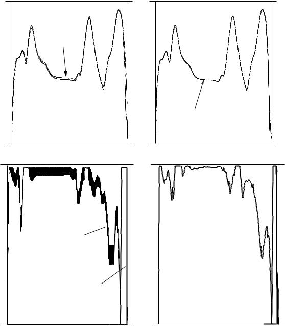
Table 6 summarizes all the 12 tests run on the at track. In addition, we present the nal performance graphs in Figure 25 for the more complex piece of real track with the same train. It shows substantial improvement in control accuracy and smoothness.

16.1.4Application Conclusions

We have presented an approach for tuning a fuzzy KB for a complex, real-world application. In particular, we used genetic algorithms to tune scaling factors as well as membership functions, and demonstrated that the approach was able to nd good solutions within a reasonable amount of time under di erent train handling criteria. In addition, we showed that all parameters do not need to be treated as equally important, and that sequential optimization can greatly reduce computational e ort by doing scaling factors rst. Additional improvement was shown by the good performance of fairly coarse encodings. The scalability of the approach enables us to customize the controller di erently for each track pro le, though it does not need to be changed for di erent train makeups. In this way, we can produce customized controllers o ine e ciently. Future extensions of this system will focus on automatic generation of velocity pro les for the train simulator by using genetic algorithms for trajectory optimization subject to \soft" constraints.

55

Figure 25: The two gures on the left show reference tracking performance and control outputs before GA tuning. After tuning, the two gures on the right show vastly improved tracking and smoothness of control. The track was a section of Selkirk|Framingham track, and the simulated train was the 9000 ton, mile-long, loaded unit train.

56

16.2Example of NN Controlled by a FLC

This example illustrates the use of a FLC to accelerate the performance of a neural network. The original problem in which it was used was the failure prediction and failure diagnostics of a complex industrial process. The details of the problem domain are still considered con dential and cannot be divulged. However, we can certainly describe the portion concerning the acceleration of the NN-based classi er.

16.2.1Neural Learning with Fuzzy Accelerators

The training method employed for neural nets in our approach is error back-propagation, which is a generalization of the Least Mean Squares (LMS) algorithm. This is essentially a gradient descent method over weight space, which seeks to minimize the mean squared error over the entire training set. Since gradient descent can be very slow, we need an acceleration technique to speed up neural learning. This is done using fuzzy rules.

As mentioned before, in section 15.1, the basic weight update equation in backpropagation is as follows:

where Wij (l) is the weight between the ith neuron at the lth layer and the jth neuron at the (l , 1)th layer, E is the sum of squared error between target and actual output, s is the iteration step, is the learning rate (usually between 0:01 and 1:0), and is the momentum coe cient (usually 0:9).

The learning rate determines how fast the algorithm will move along the error surface, following its gradient. The momentum represents the fraction of the previous changes to the weight vector Wn,1 which will stil be used to compute the current change. As implied by its name, the momentum tends to maintain the changes moving along the same direction.

From the above equation, it is clear that the e ciency of weight updating depends on the selection of the learning rate as well as the momentum coe cient. The selection of these parameters involves a tradeo : in general, large and result in fast error convergence, but poor accuracy. On the contrary, small andlead to better accuracy but slow training [Wasserman, 1989].

Unfortunately, the selections are mainly ad hoc, i.e., based on empirical results or trial and error. In addition, the choice of activation function, f(x) could also in uence the learning process:

1

f(x) = 1 + e, 12 x

where is the steepness parameter of the activation function.

The Fuzzy Accelerator used in our application is similar to that described in [Kuo et al., 1993], since ,, and are tuned simultaneously. However, the main di erence is that we use both total error andtotal training time as fuzzy premise variables for adjusting instead of using only total error. It is believed that total training time will provide the annealing e ect which yields precise convergence [Rumelhart et al., 1986]. Fuzzy rules for adjusting of and are listed in Table 7, while fuzzy rules for are shown is Table 8.

The universe of discourse of total training error is partitioned into Small, Medium, and Big, while the universe of discourse of change of error between two consecutive iterations is partitioned into Negative, Zero, and Positive. There are only nine fuzzy rules for adjustment of both the learning rate and the momentum coe cient. The point is that the training time will be reduced signi cantly even with such simple fuzzy rules. The obtained simulation results demonstrate the validity of the above argument.

Table 7: Fuzzy rule table for and .

57

In Table 8, the partitioning of total training error is the same as in Table 7, while the universe of discourse of total training time is partitioned into Short, Medium, and Long. Again, there are nine rules for adjustment of the steepness parameter of the activation function. For instance, the fuzzy rule in row 3 column 1 is interpreted as:

IF error is Small AND time for training is long THEN steepness parameter should be Large

Table 8: Fuzzy rule table for .

58

17 PART III Conclusions: Soft Computing

We should note that Soft Computing technologies are relatively young: Neural Networks originated in 1959, Fuzzy Logic in 1965, Genetic Algorithms in 1975, and probabilistic reasoning (beside the original Bayes' rule) started in 1967 with Dempster's and the in early 80s with Pearl's work. Originally, each algorithm had wellde ned labels and could usually be identi ed with speci c scienti c communities, e.g. fuzzy, probabilistic, neural, or genetic. Lately, as we improved our understanding of these algorithms' strengths and weaknesses, we began to leverage their best features and developed hybrid algorithms. Their compound labels indicate a new trend of co-existence and integration that re ects the current high degree of interaction among these scienti c communities. These interactions have given birth to Soft Computing, a new eld that combines the versatility of Fuzzy Logic to represent qualitative knowledge, with the data-driven e ciency of Neural Networks to provide ne-tuned adjustments via local search, with the ability of Genetic Algorithms to perform e cient coarse-granule global search. The result is the development of hybrid algorithms that are superior to each of their underlying SC components and that provide us with the better real-world problem solving tools.

59

References

[Adler, 1993] D. Adler. Genetic Algorithm and Simulated Annealing: A Marriage Proposal. In 1993 IEEE International Conference on Neural Networks, pages 1104{1109, San Francisco, CA., 1993.

[Agogino and Rege, 1987] A.M. Agogino and A. Rege. IDES: In uence Diagram Based Expert System.

Mathematical Modelling, 8:227{233, 1987.

[Arabshahi et al., 1992] P. Arabshahi, J.J. Choi, R.J. Marks, and T.P. Caudell. Fuzzy Control of Backpropagation. In First IEEE International Conference on Fuzzy Systems, pages 967{972, San Diego, CA., 1992.

[Armor et al., 1985] A. F. Armor, R. D. Hottenstine, I. A. Diaz-Tous, and N. F. Lansing. Cycling capability of supercritical turbines: A world wide assessment. In Fossil Plant Cycling Workshop, Miami Beach, FL, 1985.

[Badami et al., 1994] V. Badami, K.H. Chiang, , P. Houpt, and P .P. Bonissone. Fuzzy logic supervisory control for steam turbine prewarming au tomation. In Proceedings of 1994 IEEE International Conference on Fuzzy Systems, page submitted. IEEE, June 1994.

[Bayes, 1763] T. Bayes. An essay towards solving a problem in the doctrine of chances. Philosophical Transactions of the Royal Society of London, 53:370{418, 1763. (Facsimile reproduction with commentary by E.C. Molina in \Facsimiles of Two Papers by Bayes" E. Deming, Washington, D.C., 1940, New York, 1963. Also reprinted with commentary by G.A. Barnard in Biometrika, 25, 293|215, 1970.).

[Bellman and Giertz, 1973] R Bellman and M. Giertz. On the Analytic Formalism of the Theory of Fuzzy Sets. Information Science, 5(1):149{156, 1973.

[Berenji and Khedkar, 1992] H.R. Berenji and P. Khedkar. Learning and tuning fuzzy logic controllers through reinforcements. IEEE Transactions on Neural Networks, 3(5), 1992.

[Berenji and Khedkar, 1993] H.R. Berenji and P. Khedkar. Clustering in product space for fuzzy inference. In Second IEEE International conference on Fuzzy Systems, San Francisco, CA, 1993.

[Bersini et al., 1993] H. Bersini, J.P. Nordvik, and A. Bonarini. A Simple Direct Adaptive Fuzzy Controller Derived from its Neural Equivalent. In 1993 IEEE International Conference on Neural Networks, pages 345{350, San Francisco, CA., March 1993.

[Bersini et al., 1995] H. Bersini, J.P. Nordvik, and A. Bonarini. Comparing RBF and Fuzzy Inference Systems on Theoretical and Practical Basis. In 1995 International Conference on Arti cial Neural Networks (ICANN95), pages 169{174, Paris, France, Oct. 1995.

[Bezdek and Harris, 1978] J.C. Bezdek and J.O. Harris. Fuzzy partitions and relations: An axiomatic basis for clustering. Fuzzy Sets and Systems, 1:112{127, 1978.

[Bezdek, 1981] J.C. Bezdek. Pattern Recognition with Fuzzy Objective Function Algorithms. Plenum Press, New York, 1981.

[Bezdek, 1994] J.C. Bezdek. Editorial: Fuzzines vs Probability - Again (! ?). IEEE Transactions on Fuzzy Systems, 2(1):1{3, Feb 1994.

[Bonissone and Chiang, 1993] P.P. Bonissone and K.H. Chiang. Fuzzy logic controllers: From development to deployment. In Proceedings of 1993 IEEE Conference on Neural Networks, pages 610{619. IEEE, March 1993.

[Bonissone and Chiang, 1995] P. Bonissone and K. Chiang. Fuzzy logic hierarchical controller for a recuperative turbosh aft engine: from mode selection to mode melding. In J. Yen, R. Langari, and L. Zadeh, editors, Industrial Applications of Fuzzy Control and Intelligent Syste ms. Van Nostrand Reinhold, 1995.

[Bonissone and Decker, 1986] P.P. Bonissone and K. Decker. Selecting Uncertainty Calculi and Granularity: An Experiment in Trading-o Precision and Complexity. In L. N. Kanal and J.F. Lemmer, editors,

Uncertainty in Arti cial Intelligence, pages 217{247. North Holland, 1986.

60