

08.Performance of control systems
.pdf22/10/2004 |
|
|
|
|
|
|
|
|
|
8.4 |
Disturbance rejection |
|
|
|
337 |
338 |
|
|
8 Performance of control systems |
|
|
|
|
|
|
|
|
22/10/2004 |
||||||||||||||||||||||||||||||||||||||||||||
The idea here is very simple. We wish to allow a disturbance at any node which may |
|
|
|
ˆ |
to yˆ is |
|
|
|
|
|
|
|
|
|
|
|
|
|
|
|
|
|
|
|
|
|
|
|
|
|
|
|
|
|
|
|||||||||||||||||||||||||||||||||||||
the transfer function from d1 |
|
|
|
|
|
|
|
|
|
|
|
|
|
|
|
|
|
|
|
|
|
|
|
|
|
|
|
|
|
|
||||||||||||||||||||||||||||||||||||||||||
enter the system at any other node. Just where the disturbance enters a system and where |
|
|
|
|
|
|
|
yˆ(s) |
|
|
|
|
RC (s)RP (s) |
|
|
|
|
|
|
|
|
|||||||||||||||||||||||||||||||||||||||||||||||||||
it is measured can drastically change the behaviour of the system. Typically, however, one |
|
|
|
|
T1(s) = |
= |
|
|
, |
|
|
|
|
|
||||||||||||||||||||||||||||||||||||||||||||||||||||||||||
|
|
|
|
ˆ |
|
|
|
|
|
1 + R |
|
(s)R |
|
(s) |
|
|
|
|
|
|||||||||||||||||||||||||||||||||||||||||||||||||||||
measures the disturbance at the output of the interconnected system. That is, typically |
|
|
|
|
|
|
|
d1 |
(s) |
|
|
|
|
|
|
|
C |
|
|
|
|
|
P |
|
|
|
|
|
|
|
|
|
|
|
||||||||||||||||||||||||||||||||||||||
in the above discussion j is taken to be m. Before getting to an illustration by example, |
|
|
|
ˆ |
to yˆ is |
|
|
|
|
|
|
|
|
|
|
|
|
|
|
|
|
|
|
|
|
|
|
|
|
|
|
|
|
|
|
|||||||||||||||||||||||||||||||||||||
|
|
|
|
|
|
|
|
|
|
|
|
|
|
|
|
|
|
|
|
|
|
|
|
|
|
|
|
|
|
|
|
|
|
|
|
|
|
|
|
|
|
|
|
|
|
|
|
|
|
|
|
|
|
|
|
|
|
|
|
|
|
|
|
|
|
|||||||
let us provide a result which gives some obvious consequences of the notion of disturbance |
the transfer function from d2 |
|
|
|
|
|
|
|
|
|
|
|
|
|
|
|
|
|
|
|
|
|
|
|
|
|
|
|
|
|
|
|||||||||||||||||||||||||||||||||||||||||
|
|
|
|
|
|
|
|
|
|
|
|
|
|
|
|
|
|
|
|
|
|
|
|
|
|
|
|
|
|
|
|
|
|
|
|
|
|
|
||||||||||||||||||||||||||||||||||
type. The following result can be proved along the same lines as Proposition 8.11 and by |
|
|
|
|
|
yˆ(s) |
|
|
|
|
|
|
|
|
|
|
|
|
RP (s) |
|
|
|
|
|
|
|
|
|
|
|
|
|
||||||||||||||||||||||||||||||||||||||||
application of the Final Value Theorem. |
|
|
|
|
|
|
|
|
|
|
|
|
|
|
|
|
|
|
T2(s) = |
= |
|
|
|
|
|
|
|
|
|
|
|
|
|
|
|
|
|
, |
|
|
|
|||||||||||||||||||||||||||||||
|
|
|
|
|
|
|
|
|
|
|
|
|
|
|
|
|
|
ˆ |
|
1 + R |
|
(s)R |
|
|
(s)R |
|
|
(s) |
|
|
|
|||||||||||||||||||||||||||||||||||||||||
|
|
|
|
|
|
|
|
|
|
|
|
|
|
|
|
|
|
|
|
|
|
|
|
|
|
|
|
|
|
|
|
|
|
|
|
|
|
d2(s) |
|
|
|
|
|
|
|
|
|
|
C1 |
|
|
|
C2 |
|
|
|
|
|
|
P |
|
|
|
|
|
|
||||||
8.19 Proposition Let (S, G) be an IBIBO stable interconnected SISO linear system with input |
|
|
|
|
ˆ |
to yˆ is |
|
|
|
|
|
|
|
|
|
|
|
|
|
|
|
|
|
|
|
|
|
|
|
|
|
|||||||||||||||||||||||||||||||||||||||||
in node 1 and output in node m. For j {2, . . . , m} the following statements are equivalent: |
and the transfer function from d3 |
|
|
|
|
|
|
|
|
|
|
|
|
|
|
|
|
|
|
|
|
|
|
|
|
|
||||||||||||||||||||||||||||||||||||||||||||||
|
|
|
|
|
|
|
yˆ(s) |
|
|
|
|
|
|
|
|
1 |
|
|
|
|
|
|
|
|
|
|
|
|
|
|
|
|
||||||||||||||||||||||||||||||||||||||||
(i) |
(S, G) is of j-disturbance type k with input at node i; |
|
|
|
|
|
|
|
|
T3(s) = |
= |
|
|
|
|
|
|
|
|
|
|
|
|
|
|
. |
|
|
|
|
||||||||||||||||||||||||||||||||||||||||||
|
|
|
|
|
|
|
|
|
|
|
|
|
|
|
|
|
|
|
|
|
|
|
|
|
|
|
|
|
|
|
|
|
|
|||||||||||||||||||||||||||||||||||||||
|
|
|
|
|
|
|
|
|
|
|
|
|
|
|
|
|
|
|
|
|
|
|
|
|
|
|
|
|
|
|
|
|
|
|
|
|
ˆ |
(s) |
1 + R |
C |
(s)R |
P |
(s) |
|
|
|
|
|||||||||||||||||||||||||
(ii) |
limt→∞ y(t) exists and is nonzero for some j-disturbed output (d(t), y(t)) with input at |
|
|
|
|
|
|
|
d3 |
|
|
|
|
|
|
|
|
|
|
|
|
|
|
|
|
|
|
|
|
|
|
|
||||||||||||||||||||||||||||||||||||||||
|
|
|
|
|
|
|
|
|
|
|
|
|
|
|
|
|
|
|
|
|
|
|
|
|
|
|
|
|
|
|
|
|
|
|
|
|
|
|
||||||||||||||||||||||||||||||||||
|
node i, where d(t) is of type k; |
|
|
|
|
|
|
|
|
|
|
|
|
|
|
|
Let’s attach some concrete transfer functions at this point. Our transfer functions are |
|||||||||||||||||||||||||||||||||||||||||||||||||||||||
(iii) |
lims→0 |
1 |
Tji(s) exists and is nonzero. |
|
|
|
|
|
|
|
|
|
|
|
|
|||||||||||||||||||||||||||||||||||||||||||||||||||||||||
|
|
|
|
|
|
|
|
|
|
|
|
pretty artificial, but serve to illustrate the point. We take |
|
|
|
|
|
|
|
|
|
|
|
|||||||||||||||||||||||||||||||||||||||||||||||||
sk |
|
|
|
|
|
|
|
|
|
|
|
|
|
|
|
|
|
|
|
|
|
|
|
|||||||||||||||||||||||||||||||||||||||||||||||||
The preceding three equivalent statements imply the following: |
|
|
|
|
|
|
|
|
|
|
|
|
|
|
1 |
|
|
|
|
|
|
|
|
|
|
|
|
|
|
s |
|
|
|
|
|
|
|
|
|
|
||||||||||||||||||||||||||||||||
(iv) |
lim |
|
y(t) = 0 for every j-disturbed output (d(t), y(t)) with d(t) of type ` with ` < k. |
|
|
|
|
RC (s) = |
, |
|
|
RP (s) = |
|
|
. |
|
|
|
|
|
|
|
|
|||||||||||||||||||||||||||||||||||||||||||||||||
t→∞ |
|
|
|
|
|
|
|
|
|
|
|
|
|
|
|
|
||||||||||||||||||||||||||||||||||||||||||||||||||||||||
|
|
|
|
|
|
|
|
|
|
|
|
|
|
|
|
|
|
|
|
|
|
|
|
|
|
|
|
|
|
|
|
|
|
|
|
|
|
|
|
|
|
s |
|
|
|
|
|
|
|
|
|
s + 2 |
|
|
|
|
|
|
|
|
||||||||||||
Now let us consider a simple example. |
|
|
|
|
|
|
|
|
|
|
|
Check |
We compute the corresponding transfer functions to be |
|
|
|
|
|
|
|
|
|
|
|
|
|
|
|
||||||||||||||||||||||||||||||||||||||||||||
|
|
|
|
|
|
|
|
|
|
|
|
|
|
|
|
|
|
|
|
|
|
|
|
|
|
|
|
|
|
|
|
|
|
|
|
|
|
|
|
|
|
|
|
|
|
|
||||||||||||||||||||||||||
8.20 Example Let us consider the interconnected SISO linear system whose signal flow graph |
|
s2 |
|
|
|
|
s2 |
|
|
|
|
|
|
|
|
|
|
|
|
|
|
|
|
s |
|
|
|
|
s + 2 |
|||||||||||||||||||||||||||||||||||||||||||
is shown in Figure 8.17. The system has three places where disturbances ought to naturally |
TS,G(s) = |
|
, |
T1(s) = |
|
|
|
, |
|
|
T2(s) = |
|
|
|
, |
T3(s) = |
|
. |
||||||||||||||||||||||||||||||||||||||||||||||||||||||
s2 + s + 2 |
s2 + s + 2 |
|
|
s2 + s + 2 |
s2 + s + 2 |
|||||||||||||||||||||||||||||||||||||||||||||||||||||||||||||||||||
|
|
|
|
r s |
|
|
1 |
/• |
|
|
RC (s) |
|
/• |
|
RP (s) |
/• |
1 |
|
/y s |
|
A straightforward application of Proposition 8.11(iii) indicates that TS,G is of type 0. It is |
|||||||||||||||||||||||||||||||||||||||||||||||||||
|
|
|
|
ˆ( |
) |
|
|
|
|
|
f |
|
|
|
|
|
|
|
|
|
|
|
|
|
|
|
|
|
|
|
ˆ( |
) |
also easy to see from Proposition 8.19(iii) that the system is of disturbance type 2 with |
|||||||||||||||||||||||||||||||||||||||
|
|
|
|
|
|
|
|
|
|
|
|
|
|
|
|
|
|
|
|
|
|
|
|
|
|
|
|
|
|
|
|
|||||||||||||||||||||||||||||||||||||||||
|
|
|
|
|
|
|
|
|
|
|
|
|
|
|
|
|
|
|
|
|
|
|
|
|
|
|
|
|
|
|
|
|
||||||||||||||||||||||||||||||||||||||||
|
|
|
|
|
|
|
|
|
|
|
|
|
|
|
|
|
|
|
|
|
|
|
|
|
|
|
|
|
|
|
|
respect to the disturbance d1, of disturbance type 1 with respect to the disturbance d2, and |
||||||||||||||||||||||||||||||||||||||||
|
|
|
|
|
|
|
|
|
|
|
|
|
|
|
|
|
|
|
−1 |
|
|
|
|
|
|
|
|
|
||||||||||||||||||||||||||||||||||||||||||||
|
|
|
|
|
|
|
|
|
|
|
|
|
|
|
|
|
|
|
|
|
|
|
|
|
|
|
|
|
|
|
|
|
of disturbance type 0 with respect to d3. |
|
|
|
|
|
|
|
|
|
|
|
|
|
|
|
|
|
|
|
|
|
|
|
|
|
||||||||||||||
|
|
|
|
|
|
|
|
Figure 8.17 |
A system ready to be disturbed |
|
|
|
As we see in this example, the ability of a system to reject disturbances may di er |
|||||||||||||||||||||||||||||||||||||||||||||||||||||||||||
|
|
|
|
|
|
|
|
|
|
|
|
|
|
|
|
|
|
|
|
|
|
|
|
|
|
|
|
|
|
|
|
|
from the ability of a system to represent a reference signal. Furthermore, for disturbance |
|||||||||||||||||||||||||||||||||||||||
be considered, as shown in Figure 8.18. Note that one should strictly add another node to |
rejection, one typically wants the transfer function from the disturbance to the output to |
|||||||||||||||||||||||||||||||||||||||||||||||||||||||||||||||||||||||
have the property that the expected disturbance type gives zero steady-state error. Thus, |
||||||||||||||||||||||||||||||||||||||||||||||||||||||||||||||||||||||||
|
|
|
|
|
|
|
|
|
|
|
|
|
|
|
|
|
|
|
|
|
|
|
|
|
|
|
|
|
|
|
|
|
||||||||||||||||||||||||||||||||||||||||
|
|
|
|
|
ˆ |
(s) |
|
|
|
ˆ |
|
|
|
|
ˆ |
(s) |
|
|
|
|
|
|
if step disturbances are what is expected, it is su cient that the system be of disturbance |
|||||||||||||||||||||||||||||||||||||||||||||||||
|
|
|
|
|
d1 |
|
|
|
d3(s) |
|
|
|
|
d3 |
|
|
|
|
|
|
type 0. |
|
|
|
|
|
|
|
|
|
|
|
|
|
|
|
|
|
|
|
|
|
|
|
|
|
|
|
|
|
|
|
|
|
|
|
|
|||||||||||||||
|
|
|
|
|
|
|
1 |
|
|
|
|
|
|
1 |
|
|
|
|
|
|
|
1 |
|
|
|
|
|
|
|
|
|
|
|
|
|
|
|
|
|
|
|
|
|
|
|
|
|
|
|
|
|
|
|
|
|
|
|
|
|
|
|
|
|
|
||||||||
|
|
|
|
|
|
|
|
|
|
|
|
|
|
|
|
|
|
|
|
|
|
|
|
|
|
Let us look at our falling mass example thinking of the gravitational force as a distur- |
||||||||||||||||||||||||||||||||||||||||||||||
|
|
|
|
|
|
|
² RC (s) |
|
|
|
|
² |
RP |
(s) |
|
² |
|
|
|
|
|
|
||||||||||||||||||||||||||||||||||||||||||||||||||
|
|
|
|
|
|
|
|
|
|
|
|
1 |
|
|
|
|
bance. |
|
|
|
|
|
|
|
|
|
|
|
|
|
|
|
|
|
|
|
|
|
|
|
|
|
|
|
|
|
|
|
|
|
|
|
|
|||||||||||||||||||
|
|
|
|
|
|
|
|
|
|
|
|
|
/ |
|
|
|
|
|
|
/ |
|
|
/ |
|
|
|
|
|
|
|
|
|
|
|
|
|
|
|
|
|
|
|
|
|
|
|
|
|
|
|
|
|
|
|
|
|
|
|
|
|
|
|||||||||||
|
|
|
|
|
|
• |
h |
|
|
|
|
|
• |
|
|
|
|
|
|
• |
|
|
|
|
yˆ(s) |
|
|
|
|
|
|
|
|
|
|
|
|
|
|
|
|
|
|
|
|
|
|
|
|
|
|
|
|
|
|
|
|
|
|
|
|
|
||||||||||
|
|
|
|
|
|
|
|
|
|
|
|
|
|
|
|
|
|
|
|
|
|
|
|
|
|
|
|
|
|
|
8.21 Example (Example 6.60 cont’d) The block diagram for the falling mass with the grav- |
|||||||||||||||||||||||||||||||||||||||||
|
|
|
|
|
|
|
|
|
|
|
|
|
−1 |
|
|
|
|
|
|
|
|
|
|
|
|
|
|
|
||||||||||||||||||||||||||||||||||||||||||||
|
|
|
|
|
|
|
|
|
|
|
|
|
|
|
|
|
|
|
|
|
|
|
|
|
|
|
|
|
|
|
|
|
||||||||||||||||||||||||||||||||||||||||
|
|
|
|
|
|
|
|
|
|
|
Figure 8.18 Disturbances |
|
|
|
|
|
|
itational force is shown in Figure 8.19. We think of the input −mg as a disturbance input |
||||||||||||||||||||||||||||||||||||||||||||||||||||||
|
|
|
|
|
|
|
|
|
|
|
|
|
|
|
|
|
and so write d(t) = −mg1(t). This input is then a step input if we think of holding the mass |
|||||||||||||||||||||||||||||||||||||||||||||||||||||||
|
|
|
|
|
|
|
|
|
|
|
|
|
|
|
|
|
|
|
|
|
|
|
|
|
|
|
|
|
|
|
|
|
then letting it go. In fact, in our analysis, let’s agree to take y(0) = 0 and y˙(0) = 0 and see |
|||||||||||||||||||||||||||||||||||||||
the output node yˆ, but this does not change anything, so it can be safely omitted. This will |
if the controller can return the mass to y = 0 after we let it fall under gravity. The transfer |
|||||||||||||||||||||||||||||||||||||||||||||||||||||||||||||||||||||||
function from the disturbance to the output is |
|
|
|
|
|
|
|
|
|
|
|
|
|
|
|
|
|
|
|
|
||||||||||||||||||||||||||||||||||||||||||||||||||||
generally be the case for an interconnected SISO linear system. In any case, the transfer |
|
|
|
|
|
|
|
|
|
|
|
|
|
|
|
|
|
|
|
|
||||||||||||||||||||||||||||||||||||||||||||||||||||
|
|
|
|
|
|
|
|
|
|
|
|
|
|
|
|
|
|
|
|
|
|
|
|
|
|
|
|
|
|
|
|
|
|
|
|
|
|
|
||||||||||||||||||||||||||||||||||
function for the signal flow graph is |
|
|
|
|
|
|
|
|
|
|
|
|
|
|
|
|
|
|
|
|
|
|
|
|
yˆ(s) |
|
|
|
ms2 |
|
|
|
|
|
|
|
|
|
|
|
|
|
|
|
||||||||||||||||||||||||||||
|
|
|
|
|
|
|
|
|
|
|
|
|
|
|
|
|
|
|
|
|
|
|
|
|
|
|
|
|
|
|
|
|
|
|
|
|
Td(s) = |
|
|
= |
|
|
|
|
. |
|
|
|
|
|
|
|
|
|||||||||||||||||||
|
|
|
|
|
|
|
|
|
|
|
|
|
|
|
|
|
|
|
|
|
|
|
|
|
|
|
|
|
|
|
|
|
|
|
|
|
ˆ |
|
ms2 + R |
C |
(s) |
|
|
|
|
|
|
|
|
|||||||||||||||||||||||
|
|
|
|
|
|
|
|
|
|
|
|
|
|
yˆ(s) |
|
|
|
|
RC (s)RP (s) |
|
|
|
|
|
|
|
|
|
|
|
|
|
d(s) |
|
|
|
|
|
|
|
|
|
|
|
|
|
|
|
|
|
|
|
|
|||||||||||||||||||
|
|
|
|
|
|
|
|
|
TS,G(s) = |
= |
|
|
|
, |
|
|
|
|
|
|
|
|
|
|
|
|
|
|
|
|
|
|
|
|
|
|
|
|
|
|
|
|
|
|
|
|
|
|
|
|
|
|
|
|
|
|
||||||||||||||||
|
|
|
|
|
|
|
|
|
rˆ(s) |
1 + RC (s)(s)RP (s) |
|
|
|
Let us look at the form of this transfer function for the various controllers we employed in |
||||||||||||||||||||||||||||||||||||||||||||||||||||||||||
|
|
|
|
|
|
|
|
|
|
|
|
|
|
|
|
|
|
|
||||||||||||||||||||||||||||||||||||||||||||||||||||||
Example 6.60.

22/10/2004 |
8.4 Disturbance rejection |
339 |
−mg
rˆ(s) |
RC (s) |
1 |
yˆ(s) |
|
ms2 |
||||
|
− |
|
Figure 8.19 Block diagram for falling mass with gravitational force
1. With proportional control we have RC (s) = K and so
ms2 Td(s) = ms2 + K .
This transfer function has poles on the imaginary axis, and so is not a candidate for having its type defined. Nonetheless, we can compute the time response using Proposition 3.40
ˆ |
mg |
. We ascertain that the output to this disturbance is |
given d(s) = − s |
||
r
K yd(t) = −mg cos mt.
One can see that the system does not respond very nicely in this case to the step disturbance, and to further illustrate the point, we plot this step response in Figure 8.20 for
|
10 |
|
|
|
|
|
5 |
|
|
|
|
(t) |
0 |
|
|
|
|
Σ |
|
|
|
|
|
1 |
|
|
|
|
|
|
-5 |
|
|
|
|
|
-10 |
|
|
|
|
|
1 |
2 |
3 |
4 |
5 |
|
|
|
t |
|
|
Figure 8.20 Response of falling mass to step disturbance with proportional control
m = 1, g = 9.81, and K = 28.
2. For derivative control we take RC (s) = KTDs which gives
ms
Td(s) = ms + KTD .
This disturbance transfer function is type 1 and so the steady-state disturbance to the step input d(t) = −mg is zero. Using Proposition 3.40 we determine that the response is
yd(t) = −mge−KTDt/m
340 |
8 Performance of control systems |
22/10/2004 |
|
2 |
|
|
|
|
|
0 |
|
|
|
|
|
-2 |
|
|
|
|
(t) |
-4 |
|
|
|
|
Σ |
|
|
|
|
|
1 |
|
|
|
|
|
|
-6 |
|
|
|
|
|
-8 |
|
|
|
|
|
1 |
2 |
3 |
4 |
5 |
|
|
|
t |
|
|
Figure 8.21 Response of falling mass to step disturbance with derivative control
and we plot this response in Figure 8.21 for m = 1, g = 9.81, K = 28, and TD = 289 . Note that this response decays to zero which is consistent with our observation that the error to a step disturbance should decay to zero in the steady-state.
3. If we use an integral controller we take RC (s) = 1 from which we compute
TI s
mTI s3 Td(s) = mTI s3 + K .
To examine this transfer function for type, let us be concrete and choose m = 1, g = 9.81, K = 28, TD = 289 , and TI = 107 . One determines (Mathematica®!) that the roots of
mTI s3 + K are then |
√3 5 ± |
√3√3 5i, −2√3 5. |
|
Since the transfer function has poles in C+, the notion of type is not applicable. We plot the response to the step gravitational disturbance in Figure 8.22, and we see that it is
|
10000 |
|
|
|
|
|
7500 |
|
|
|
|
|
5000 |
|
|
|
|
(t) |
2500 |
|
|
|
|
0 |
|
|
|
|
|
Σ |
|
|
|
|
|
1 |
|
|
|
|
|
|
-2500 |
|
|
|
|
|
-5000 |
|
|
|
|
|
-7500 |
|
|
|
|
|
1 |
2 |
3 |
4 |
5 |
|
|
|
t |
|
|
Figure 8.22 Response of falling mass to step disturbance with integral control
badly behaved. Thus the given integral controller will magnify the disturbance.

22/10/2004 |
8.4 Disturbance rejection |
341 |
4. Finally we combine the three controllers into a nice PID control law: RC (s) = K +
KTDs + K . The disturbance to output transfer function is then
TIs
mTI s3
Td(s) = mTI s3 + KTDTI s2 + KTI s + K .
For our parameters m = 1, g = 9.81, K = 28, TD = 289 , and TI = 107 , we determine that the roots of the denominator polynomial are −5, −2 ± 2i (recall that we had chosen the PID parameters in just this way). Since these roots are all in C−, we may make the observation that the disturbance type is 3. Therefore the steady-state error to a step disturbance should be zero. The response of this transfer function to the gravitational step disturbance is shown in Figure 8.23 for m = 1, g = 9.81, K = 28, TD = 289 , and
|
2 |
|
|
|
|
|
0 |
|
|
|
|
(t) |
-2 |
|
|
|
|
|
|
|
|
|
|
Σ |
-4 |
|
|
|
|
1 |
|
|
|
|
|
|
-6 |
|
|
|
|
|
-8 |
|
|
|
|
|
1 |
2 |
3 |
4 |
5 |
|
|
|
t |
|
|
Figure 8.23 Response of falling mass to step disturbance with PID control
TI = 107 . This response decays to zero as it ought to.
Let us address the question of how to interpret our computations for the gravitational disturbance to the falling mass. One needs to be careful not to misinterpret the disturbance response for the system response. The input/output response of the system for the various controllers was already investigated in Example 6.60. When examining the system including the e ects of the disturbance, one must take into account both the input/output response and the response to the disturbance.
For example, with the PID controller we had chosen, our analysis of both these responses suggests that the system with the chosen parameters should behave nicely with the gravitational force. To verify this, let us look at the situation where we hold the mass still at y = 0 and at time t = 0 let it go. Our PID controller is then charged with bringing the mass back to y = 0. The initial value problem governing this situation is
my¨ + KTDy˙(t) + Ky(t) + TI Z0 |
t |
y(0) = 0, y˙(0) = 0. |
|||
y(τ) dτ = −mg, |
|||||
|
|
K |
|
|
|
To solve this equation we di erentiate once to get the initial value problem |
|||||
... |
K |
|
y˙(0) = 0, y¨(0) = −g. |
||
my + KTDy¨(t) + Ky˙(t) + |
|
y(t) = 0, y(0) = 0, |
|||
TI |
|||||
smooth this
342 |
8 Performance of control systems |
22/10/2004 |
|
0.1 |
|
|
|
|
|
0.05 |
|
|
|
|
|
0 |
|
|
|
|
(t) |
-0.05 |
|
|
|
|
-0.1 |
|
|
|
|
|
y |
|
|
|
|
|
|
-0.15 |
|
|
|
|
|
-0.2 |
|
|
|
|
|
-0.25 |
|
|
|
|
|
1 |
2 |
3 |
4 |
5 |
|
|
|
t |
|
|
Figure 8.24 Response of falling mass with PID controller
The solution is plotted in Figure 8.24 for the chosen PID parameters. As should be the case, the response is nice with the PID controller bringing the mass back to its initial height in relatively short order.
This example is one which contains a lot of information, so you would be well served to spend some time thinking about it.
8.5 The sensitivity function
In this section we introduce and study a transfer function which is, at least for certain block diagram configurations, “complementary” to the transfer function. The block diagram configuration we look at is the one we first looked at in Section 6.3.2, and the configuration is reproduced in Figure 8.25. One may extend the discussion here to more general block
eˆ(s) |
ˆ |
|
d(s) |
rˆ(s) 


 RL(s)
RL(s) 

 yˆ(s)
yˆ(s)
−

 nˆ(s)
nˆ(s)
Figure 8.25 Block diagram for investigating the sensitivity function
diagram configurations, but this unity gain feedback setup is one which can be handled nicely. In this scenario, we are typically supposing that the loop gain RL is the product of a plant transfer function RP and a controller transfer function RC . But unless we say otherwise, we just take RL as a transfer function in its own right, and do not concern ourselves with from where it comes.
22/10/2004 |
8.5 The sensitivity function |
343 |
8.5.1 |
Basic properties of the sensitivity function Let us first make some elementary |
|
observations concerning the closed-loop transfer function and the sensitivity function. The following result follows immediately from the definition of TL and SL.
8.22 Proposition For the feedback interconnection of Figure 9.3, the following statements hold:
(i)p C is a pole for RL if and only if SL(p) = 0 and TL(p) = 1;
(ii)z C is a zero for RL if and only if SL(z) = 1 and TL(z) = 0.
The import of this simple result is that it holds for any loop gain RL. Thus the zeros and poles for RL are immediately reflected in the closed-loop transfer function and the sensitivity function. Let us introduce the following notation:
Z(SL) = {s C | SL(s) = 0}
(8.2)
Z(TL) = {s C | TL(s) = 0} .
This notation will be picked up again in Section 9.2.1.
Let us illustrate this with an example some of the simpler features of the sensitivity function.
8.23 Example (Example 6.60 cont’d) Let us carry on with our falling mass example. What we shall do is plot the frequency response of the closed-loop transfer function and the sensitivity function on the same Bode plot. We have RL(s) = RC (s)ms1 2 , and we shall use the four controller transfer functions of Example 6.60. In all cases, we take m = 1.
1. We take RC (s) = K with K = 28. In Figure 8.26 we give the Bode plots for the closed-
|
30 |
10 |
|
20 |
5 |
|
0 |
|
|
10 |
|
|
-5 |
|
|
|
|
dB |
0 |
dB-10 |
|
-10 |
-15 |
|
-20 |
|
|
-20 |
|
|
-25 |
|
|
|
|
|
-1.5 -1 -0.5 0 0.5 1 1.5 2 |
-1.5 -1 -0.5 0 0.5 1 1.5 2 |
|
log ω |
log ω |
|
150 |
|
|
|
|
|
|
|
|
150 |
|
|
|
|
|
|
|
|
100 |
|
|
|
|
|
|
|
|
100 |
|
|
|
|
|
|
|
deg |
50 |
|
|
|
|
|
|
|
deg |
50 |
|
|
|
|
|
|
|
0 |
|
|
|
|
|
|
|
0 |
|
|
|
|
|
|
|
||
|
|
|
|
|
|
|
|
|
|
|
|
|
|
|
|
||
|
-50 |
|
|
|
|
|
|
|
|
-50 |
|
|
|
|
|
|
|
|
-100 |
|
|
|
|
|
|
|
|
-100 |
|
|
|
|
|
|
|
|
-150 |
|
|
|
|
|
|
|
|
-150 |
|
|
|
|
|
|
|
|
-1.5 |
-1 |
-0.5 |
0 |
0.5 |
1 |
1.5 |
2 |
|
-1.5 |
-1 |
-0.5 |
0 |
0.5 |
1 |
1.5 |
2 |
log ω |
log ω |
Figure 8.26 Bode plots for the closed-loop transfer function and sensitivity function for the falling mass with proportional controller (left) and derivative controller (right). In each case, the solid line represents the closed-loop transfer function and the dashed line the sensitivity function.
loop transfer function (the solid line) and the sensitivity function (the dashed line).
344 |
8 Performance of control systems |
22/10/2004 |
2.Next we take RC (s) = KTDs with K = 28 and TD = 289 . In Figure 8.26 we give the Bode plots for the closed-loop transfer function and the sensitivity function.
3. Now we consider pure integral control with RC (s) = |
1 |
with TI = |
7 |
. In Figure 8.26 we |
|
TI s |
10 |
||||
|
|
|
10 |
5 |
0 |
-5 |
dB-10 |
-15 |
-20 |
-25 |
dB
10
5
0 -5
-5
-10 -15 -20 -25
|
-1.5 |
-1 |
-0.5 |
0 |
0.5 |
1 |
1.5 |
2 |
|
-1.5 |
-1 |
-0.5 |
0 |
0.5 |
1 |
1.5 |
2 |
|
|
|
log ω |
|
|
|
|
|
|
|
log ω |
|
|
|
|
||
|
150 |
|
|
|
|
|
|
|
|
150 |
|
|
|
|
|
|
|
|
100 |
|
|
|
|
|
|
|
|
100 |
|
|
|
|
|
|
|
deg |
50 |
|
|
|
|
|
|
|
deg |
50 |
|
|
|
|
|
|
|
0 |
|
|
|
|
|
|
|
0 |
|
|
|
|
|
|
|
||
|
|
|
|
|
|
|
|
|
|
|
|
|
|
|
|
||
|
-50 |
|
|
|
|
|
|
|
|
-50 |
|
|
|
|
|
|
|
|
-100 |
|
|
|
|
|
|
|
|
-100 |
|
|
|
|
|
|
|
|
-150 |
|
|
|
|
|
|
|
|
-150 |
|
|
|
|
|
|
|
|
-1.5 |
-1 |
-0.5 |
0 |
0.5 |
1 |
1.5 |
2 |
|
-1.5 |
-1 |
-0.5 |
0 |
0.5 |
1 |
1.5 |
2 |
|
|
|
log ω |
|
|
|
|
|
|
|
log ω |
|
|
|
|
||
Figure 8.27 Bode plots for the closed-loop transfer function and sensitivity function for the falling mass with integral controller (left) and PID controller (right). In each case, the solid line represents the closed-loop transfer function and the dashed line the sensitivity function.
give the Bode plots for the transfer function (the solid line) and the sensitivity function (the dashed line).
4. Finally, we look at a PID controller so that RC (s) = K + KTDs + |
1 |
, and we use the |
TIs |
same numerical values as above. As expected, in Figure 8.27 you will find the Bode plots for the closed-loop transfer function and the sensitivity function.
In all cases, note that the gain attenuation at high frequencies leads to high sensitivities at these frequencies, and all the associated disadvantages.
8.5.2 Quantitative performance measures Our emphasis to this point has been essentially on descriptive measures of performance. However, it is very helpful to have on hand quantitative measures of performance. Indeed, such performance measures form the backbone of modern control theory, as from these precise performance characteristics spring useful design methodologies. The reader will wish to recall from Section 5.3.1 the definitions of the L2 and L∞-norms.
The quantitative measures we will provide are those on the error of a system to a step input. Thus we work with the block diagram of Figure 6.25 which we reproduce in Figure 8.28. We shall assume that the closed-loop system is type 1 so that the steady-state error to a step input is zero. In order to make meaningful comparisons, we deal with the unit step response to the reference 1(t).
For design methodologies with a mathematical basis, the following two measures of per-

22/10/2004 |
8.5 The sensitivity function |
345 |
346 |
8 Performance of control systems |
22/10/2004 |
8.6 Frequency-domain performance specifications
The time-domain performance specifications of Section 8.1 are traditionally what one
rˆ(s) RL(s) yˆ(s) encounters as these are the easiest to achieve a feeling for. However, there are powerful
−
controller design methods which rely on specifying the performance requirements in the frequency-domain, not the time-domain. In this section we address this in two ways. First we look at some specifications that are actually most naturally given in the frequencydomain. These are followed by an explanation of how time-domain specifications can be
approximately turned into frequency-domain specifications.
Figure 8.28 Block diagram for quantitative performance measures
|
|
|
|
|
|
|
|
|
|
|
|
|
|
|
|
8.6.1 |
|
Natural frequency-domain specifications There are a significant number of |
||||||||||
formance are often the most useful: |
|
|
|
|
|
|
|
|
|
|
|
|
performance specifications that are very easily presented in the frequency-domain. In this |
|||||||||||||||
|
|
|
|
|
|
|
|
|
|
|
|
section we list some of these. In a given design problem, one may wish to invoke only some |
||||||||||||||||
|
|
|
|
∞ |
|
|
|
|
|
1/2 |
|
|
|
|
|
|||||||||||||
|
|
|
|
|
|
|
|
|
|
|
|
of these constraints and not others. Also, the exact way in which the specifications are best |
||||||||||||||||
kek2 = |
Z0 |
e |
2 |
(t) dt |
|
|
|
|
|
|
|
|||||||||||||||||
|
|
|
|
|
|
|
|
presented can vary in detail, depending on the particular application. However, it can be |
||||||||||||||||||||
kek∞ = sup{|e(t)| ≤ α for almost every t}. |
|
hoped that what we say here is a helpful guide in getting started in a given problem. |
||||||||||||||||||||||||||
|
α≥0 |
|
|
|
|
|
|
|
|
|
|
|
Before we begin, we remark that all of the specifications we give will be are what Helton |
|||||||||||||||
The first is of course the L2-norm of the error, and the second the L∞-norm of the error. |
|
and Merrino [1998] call “disk constraints.” This means that the closed-loop transfer function |
||||||||||||||||||||||||||
|
TL will be specified to satisfy a constraint of the form |
|
||||||||||||||||||||||||||
The error measure |
|
|
|
kek1 = Z0 ∞ |e(t)| dt |
|
|
|
|
|
|||||||||||||||||||
|
|
|
|
|
|
|
|
|
|
|
|
|
|
|
|
|
|
|
|
|||||||||
|
|
|
|
|
|
|
|
|
|
|M(iω) − TL(iω)| ≤ R(iω), ω [ω1, ω2] |
|
|||||||||||||||||
is also used. For example, you will recall from Section 13.1 that the criterion used by Ziegler |
R+ defined? |
for functions M : i[ω1, ω2] → C M : i[ω1, ω2] → R+, and for ω1 < ω2 > 0. |
Thus at each |
|||||||||||||||||||||||||
and Nicols in their PID tuning was the minimisation of the L |
1 |
-norm. In practice, one will |
||||||||||||||||||||||||||
|
|
frequency ω in the interval [ω1, ω2], the value of TL at iω must lie in the disk of radius R(iω) |
||||||||||||||||||||||||||
sometimes wish to consider alternative performance measures. For example, the following |
|
with centre M(iω). |
|
|
|
|
|
|
|
|
|
|
||||||||||||||||
two, related to the L2 and L1-norms, will serve to penalise errors which occur for large times, |
|
|
|
|
|
|
|
|
|
|
|
|
|
|
||||||||||||||
but deemphasise large initial errors: |
|
|
|
|
|
|
|
|
|
|
|
Stability margin lower bound Recall from Proposition 7.15 that the point on the Nyquist |
||||||||||||||||
|
|
|
|
|
|
|
|
|
|
|
|
|
|
|
|
|||||||||||||
|
k |
e |
kt,2 |
= |
|
∞ |
2 |
1/2 |
|
|
|
contour closest to −1 + i0 is a distance kSLk∞ away. Thus, to improve stability margins, |
||||||||||||||||
|
|
|
te (t) dt |
|
|
|
|
one should provide a lower bound for this distance. This means specifying an upper bound |
||||||||||||||||||||
|
|
|
|
Z0 |
|
|
|
|
|
|
|
on the H |
|
-norm of the sensitivity function. In terms of the transfer function this gives |
||||||||||||||
|
kekt,1 = Z0 |
∞ t |e(t)| dt. |
|
|
|
|
|
∞ |
| |
1 |
− |
TL(iω) |
| ≤ |
ρsm, |
|
|
ω > 0. |
(8.3) |
||||||||||
|
|
|
|
|
|
|
|
|
|
|
|
|
|
|
|
|
|
|
|
|
|
|
|
|
||||
One can imagine choosing other weighting functions of time by which to multiply the error |
|
It is possible that one may wish to enforce this constraint more or less at various frequencies. |
||||||||||||||||||||||||||
to suit the particular nature of the problem with which one is dealing. |
|
|||||||||||||||||||||||||||
|
For example, if one knows that a system will be operating in a certain frequency range, then |
|||||||||||||||||||||||||||
One of the reasons for the usefulness of the L2 and L∞ norms is that they make it possible |
|
|||||||||||||||||||||||||||
|
stability margins in this frequency range will be more important that in others. Thus one |
|||||||||||||||||||||||||||
to formulate statements in terms of transfer functions. For example, we have the following |
|
|||||||||||||||||||||||||||
|
may relax (8.3) by introducing a weighting function W and asking that |
|
||||||||||||||||||||||||||
result which was derived in the course of the proof of Theorem 5.22, if we recall that the |
|
|
||||||||||||||||||||||||||
|
|
|
|
|
|
|
|
|
|
|
|
|
|
|||||||||||||||
transfer function from the input to the error in Figure 8.28 is the sensitivity function. |
|
|
|
|W (iω)(1 − TL(iω))| ≤ ρsm, |
|
ω > 0, ω > 0. |
|
|||||||||||||||||||||
|
|
|
|
|
|
|
|
|
|
|
|
|
|
|
|
|
|
|
|
|||||||||
8.24 Proposition Consider the block diagram of Figure 8.28 and suppose that the closed-loop |
|
As a disk constraint this reads. |
|
|
|
|
|
|
|
|
|
|
||||||||||||||||
system is type k for k ≥ 1. If e(t) is the error to an input u L2[0, ∞), then |
|
|
|
|1 − TL(iω)| ≤ |
|
ρsm |
|
, |
ω > 0. |
(8.4) |
||||||||||||||||||
|
|
|
|
kek2 ≤ kSLk∞ kuk2 . |
|
|
|
|
|
|
|W (iω)| |
|||||||||||||||||
where SL is the sensitivity function of the closed-loop system. |
|
|
|
Tracking specifications Recall that the tracking error is minimised as in Proposition 8.24 |
||||||||||||||||||||||||
|
|
|
by minimising kSLk∞. However, the kind of tracking error minimisation demanded by |
|||||||||||||||||||||||||
This proposition tells us that if a design objective is to minimise the transfer of energy |
|
|||||||||||||||||||||||||||
|
Proposition 8.24 is extremely stringent. |
Indeed, |
it |
asks that for any sort |
of input, we |
|||||||||||||||||||||||
from the input signal to the error signal, then one should aim to minimise the H∞-norm of |
|
minimise the L2-norm of the error. |
However, in practice one will wish to minimise the |
|||||||||||||||||||||||||
SL.

22/10/2004 8.6 Frequency-domain performance specifications 347
tracking error for inputs having a certain frequency response. To this end, we may specify various sorts of specifications that are less restrictive than minimising kSLk∞.
A first case we consider is a constraint |
|
|1 − TL(iω)| < Rtr, ω [ω1, ω2]. |
(8.5) |
This corresponds to tracking well signals whose frequency response is predominantly supported in the given range.
Another approach that may be taken occurs when one knows, or approximately knows, the transfer function for the reference one wishes to track. That is, suppose that we wish to track the reference r(t) whose Laplace transform is rˆ(s). Generalising the analysis of Section 8.3 in a straightforward way from type k reference signals to reference signals with a general Laplace transform, we see that to track r well we should require
|(1 − TL(iω))ˆr(iω)| ≤ ρtr, |
ω [ω1, ω2]. |
|
||
This is then made into the disk constraint |
|
|
|
|
|1 − TL(iω)| ≤ |
ρtr |
, |
ω [ω1, ω2]. |
(8.6) |
|rˆ(iω)| |
||||
Bandwidth constraints One of the more important features of a closed-loop transfer function is its bandwidth. As we saw in Section 8.2, larger bandwidth generally means quicker response. However, one wishes to limit the bandwidth since it is often destructive to a system’s physical components to have the response to high-frequency signals not be adequately attenuated.
Let us take this opportunity to define bandwidth for fairly general systems. Motivated by our observations for first and second-order transfer functions, we make the following definition.
8.25 Definition Let (N, D) be a proper SISO linear system in input/output form and let
|
kTN,Dk∞ |
= ω {| |
H |
N,D |
|
|} |
||
|
|
|
|
sup |
|
(ω) , |
||
as usual. When limω→0 |HN,D(ω)| < ∞, we consider the following five cases: |
||||||||
(i) |
(N, D) is strictly proper and steppable: the bandwidth of (N, D) is defined by |
|||||||
|
ωN,D = ω¯ |
|
|
HN,D(ω) |
|
|
|
|
|
||HN,D(0)|| ≤ √2 |
|||||||
|
inf |
ω¯ |
|
|
|
|
1 |
for all ω > ω¯ ; |
(ii) |
(N, D) is not strictly proper and |
not steppable: the bandwidth of (N, D) is defined |
||||||
|
|
|
|
|
|
|||
|
by |
|
|
|
|
|
|
|
|
|
HN,D(ω) |
|
|
||||
|
ωN,D = ω¯ |
||HN,D(∞)|| |
≤ |
√2 |
||||
|
sup |
ω¯ |
|
|
|
|
1 |
for all ω < ω¯ ; |
(iii)(N, D) is strictly proper, not steppable, and kTN,Dk∞ < ∞: the lower cuto frequency of (N, D) is defined by
ωN,D |
= ω¯ |
ω¯ |
|
HN,D(ω) |
≤ |
√2 |
|
|
|
|||
|kTN,Dk∞| |
|
|
||||||||||
lower |
sup |
|
|
|
|
|
|
1 |
|
for all ω < ω¯ |
||
and the upper cuto frequency |
of (N, D) is defined by |
|
||||||||||
ωN,Dupper = inf |
ω¯ |
|
|HN,D(ω)| |
√1 |
|
for all ω > ω¯ |
, |
|||||
|
ω¯ |
|
|
k |
TN,Dk∞ ≤ |
2 |
|
|
|
|||
|
|
|
upper |
− |
ω |
lower |
; |
|||||
and the bandwidth is given by ωN,D = ω |
N,D |
N,D |
|
|||||||||
|
|
|
|
|
|
|
|
|
||||
bandwidth and gain crossover frequency
348 |
8 Performance of control systems |
22/10/2004 |
(iv) |
(N, D) is strictly proper, not steppable, and kTN,Dk∞ = ∞: the bandwidth of (N, D) |
|
|
is not defined; |
|
(v) |
(N, D) is not strictly proper and steppable: the bandwidth of (N, D) is not defined. |
|
When limω→0 |HN,D(ω)| = ∞, bandwidth is undefined. |
|
|
Thus ωN,D is, for “typical” systems, simply the frequency at which the magnitude part of the Bode plot drops below, and stays below, the DC value minus −3dB. For most other transfer functions, definition of bandwidth is still possible, but must be modified to suit the characteristics of the system. Note that the bandwidth is not defined for systems with imaginary axis poles. However, this is not an issue since such systems are not BIBO stable, and we are typically interested in bandwidth for the closed-loop transfer function, where BIBO stability is essential.
With is general notion of bandwidth, the typical bandwidth constraint one may pose might take the form
|TL(iω)| < ρbw, ω > ωbw. |
(8.7) |
High-frequency roll-o In practise one does not want the closed-loop transfer function to be proper, but strictly proper. This will ensure that the system will not be overly susceptible to high-frequency disturbances in the reference. Furthermore, one will often want the closedloop transfer function to not only be proper, but to have a certain relative degree, so that it falls o at a prescribed rate as ω → ∞. Note that
TL(iω) = |
RC (iω)RP (iω) |
. |
|
||
|
1 + RC (iω)RP (iω) |
|
Therefore, assuming that RC RP is proper, for large frequencies TL(iω) behaves like RC (iω)RP (iω). To render the desired behaviour as a disk inequality, we first assume that we insist on controllers that satisfy an inequality of the form
ρC
|RC (iω)| ≤ |ω|nC
for some ρC > 0 and nC N. This is tantamount to making a relative degree constraint on the controller. Since we are primarily concerned with high-frequency behaviour, the choice of ρC is not critical. Assuming that such a constraint has been enforced, the high-frequency approximation
|
|
|
TL(iω) ≈ RC (iω)RP (iω) |
|
|
||||
gives rise to the inequality |
|
|
|
|
|
|
|
|
|
| |
T |
|
(iω) |
| ≤ |
ρC |RP (iω)| |
, |
[ω |
, ω ]. |
(8.8) |
|
L |
|
|ω|nC |
1 |
2 |
|
|||
Controller output constraints |
The transfer function |
|
|
|
|||||
RC
RC SL = 1 + RC RP
is sometimes called the closed-loop controller. It is the transfer function from the error to the output from the plant. One would wish to minimise this transfer function in order to ensure that the controller is not excessively aggressive. In practise, an excessively aggressive
22/10/2004 |
8.6 Frequency-domain performance specifications |
349 |
350 |
8 Performance of control systems |
22/10/2004 |
controller might cause saturation, i.e., the controller may not physically be able to supply the output needed. Saturation is a nonlinear e ect, and should be avoided, unless its e ects are explicitly accounted for in the modelling.
In any event, the constraint we consider to limit the output of the closed-loop controller
is
|RC (iω)(1 − TL(iω))| ≤ ρclc,
Overshoot attenuation In Section 8.2.2 we saw that there is a relationship, at least for second-order transfer functions, between a peak in the frequency response for the closed-loop transfer function and a large overshoot. While no theorem to this e ect is known to the author, it may be desirable to enforce a constraint on kTLk∞ of the type
|TL(iω)| ≤ ρos, ω ≥ 0. |
(8.11) |
where we leave the frequency unspecified for the moment. Using the relation |
|
Summary We have given a list of “typical” frequency-domain constraints. In practise one |
|||||||||||||||||||||
|
|
|
|
|
|
|
|
|
|
|
|
|
|
|
|
|
|
|
|
|
|||
|
TL = |
|
RC RP |
|
= RC RP = |
|
TL |
|
, |
|
rarely enforce all of these simultaneously. Nevertheless, in a given application, any of the |
||||||||||||
|
1 + R |
|
R |
|
1 |
− |
T |
|
|
constraints (8.3), (8.4), (8.5), (8.6), (8.8), (8.7), (8.9), (8.10), or (8.11) may prove useful. |
|||||||||||||
this gives the disk constraint |
|
|
C |
|
P |
|
|
|
|
|
|
L |
|
Note that specifying the constants and various weighting functions will be a process of trial |
|||||||||
|
|TL(iω)| ≤ ρclc |RP (iω)| . |
|
|
|
|
|
and error in order to ensure that one specifies a problem that is solvable, and still has |
||||||||||||||||
|
|
|
|
|
|
|
|
|
|
satisfactory performance. In Chapter 9 we discuss in detail the idea that not all types of |
|||||||||||||
Now let us turn our attention to the reasonable ranges of frequency for the invocation of |
frequency-domain performance specification should be expected to be achievable, particu- |
||||||||||||||||||||||
larly for unstable and/or nonminimum phase plants. The methods for obtaining controllers |
|||||||||||||||||||||||
such a constraint. Clearly the constraint will have the greatest e ect for frequencies that are |
|||||||||||||||||||||||
satisfying the type of frequency-domain constraints we have discussed in this section may be |
|||||||||||||||||||||||
zeros for RP that are on the imaginary axis. This we let iz1, . . . , izk be the imaginary axis |
|||||||||||||||||||||||
found in the book [Helton and Merrino 1998], where a software is demonstrated for doing |
|||||||||||||||||||||||
zeros for RP , and take as our disk constraint |
|
|
|
|
|
|
|
|
|
|
|||||||||||||
|
|
|
|
|
|
|
|
|
|
such design. This is given further discussion in Chapter 15 in terms of “H∞ methods.” |
|||||||||||||
|TL(iω)| ≤ ρclc |RP (iω)| , |
|
ω [z1 − r1, z1 + r1] · · · [zk − rk, zk + rk], |
(8.9) |
||||||||||||||||||||
|
|
8.6.2 Turning time-domain specifications into frequency-domain specifications It |
|||||||||||||||||||||
for some r1, . . . , rk > 0. |
|
|
|
|
|
|
|
|
|
|
|
|
|
|
|
|
|
|
|
|
|||
|
|
|
|
|
|
|
|
|
|
|
|
|
|
|
|
|
|
|
is generally not possible to make a given time-domain performance specification and pro- |
||||
|
|
|
|
|
|
|
|
|
|
|
|
|
|
|
|
|
|
|
|
|
duce an exact, tractable frequency-domain specification. Nonetheless, one can make some |
||
Plant output constraints The idea here is quite similar to that for the closed-loop con- |
progress in producing reasonably e ective and manageable frequency-domain specifications |
||||||||||||||||||||||
troller. To wit, the name closed-loop plant is often given to the transfer function |
|
from many types of time-domain specifications. The idea is to produce a transfer func- |
|||||||||||||||||||||
|
|
|
|
|
|
|
|
|
|
|
RP |
|
|
|
|
|
|
tion having the desired time-domain behaviour, then using this as the basis for forming the |
|||||
|
|
|
|
|
|
|
|
|
|
|
|
|
|
|
finish |
frequency-domain specifications. |
|||||||
|
|
|
|
|
|
RP SL = 1 + RC RP . |
|
|
|
|
|||||||||||||
|
|
|
|
|
|
|
|
|
|
|
|
|
|||||||||||
This is the transfer function from the output of the controller to the output of the plant. |
|
8.7 Summary |
|||||||||||||||||||||
That this should be kept from being too large is a reflection of the desire to not have the |
|
|
|||||||||||||||||||||
plant “overreact” to the controller. |
|
|
|
|
|
|
|
|
|
|
|
|
|
|
|
|
When designing a controller the first step is typically to determine acceptable perfor- |
||||||
The details of the computation of the ensuing disk constraint go very much like that for |
mance criterion. In this chapter, we have come up with a variety of performance measures. |
||||||||||||||||||||||
the closed-loop controller. We begin by considering the constraint |
|
Let us review what we have said. |
|||||||||||||||||||||
|
|
|
|
|
|RP (iω)(1 − TL(iω))| ≤ ρclp, |
|
|
|
|
|
1. Based upon a system’s step response, we defined various performance features (rise time, |
||||||||||||
|
|
|
|
|
|
|
|
|
|
|
overshoot, etc.). These features should be understood at least in that one should be able |
||||||||||||
immediately giving rise to the disk constraint |
|
|
|
|
|
|
|
|
|
|
|
to compare two signals and determine which is the better with respect to certain of these |
|||||||||||
|
|
|
|
|
|
|
|
|
|
|
performance features. |
||||||||||||
|
|
|
|
|
|
|
|
|
|
|
|
ρclp |
|
|
|
|
|
|
|
||||
|
|
|
|
|
|
|
|
|
|
|
|
|
|
|
|
|
2. Some of the character of system response are exhibited by a simple second-order transfer |
||||||
|
|
|
|
|
|1 − TL(iω)| ≤ |RP (iω)|. |
|
|
|
|
|
|||||||||||||
|
|
|
|
|
|
|
|
|
|
|
function. In particular, the tradeo s one has to make in controller design begin to show |
||||||||||||
To determine when one should invoke this constraint, note that it most restrictive for fre- |
|
up for such systems in that one cannot perfectly satisfy all performance measures. |
|||||||||||||||||||||
3. For simple systems, often one can obtain an adequate understanding of the problems to |
|||||||||||||||||||||||
quencies near imaginary axis poles for RP . |
Thus we let p1, . . . , pk be the imaginary axis |
||||||||||||||||||||||
|
be encountered in system performance by using the observations seen when additional |
||||||||||||||||||||||
poles for RP and take the constraint |
|
|
|
|
|
|
|
|
|
|
|
|
|
|
|
||||||||
|
|
|
|
|
|
|
|
|
|
|
|
|
|
|
poles and zeros are added to a second-order transfer function. |
||||||||
|
|
ρclp |
|
|
|
|
|
|
|
|
|
|
|
|
|
|
|
|
|
|
|||
|1 − TL(iω)| ≤ |
|
|
, ω [p1 − r1 |
, p1 + r1] · · · [pk − rk, pk + rk], |
(8.10) |
4. |
The e ects of the existence of unstable poles and nonminimum phase zeros on the step |
||||||||||||||||
R |
|
(iω) |
|
||||||||||||||||||||
| |
P |
|
| |
|
|
|
|
|
|
|
|
|
|
|
|
|
|
|
|
response should be understood. |
|||
for given r1, . . . , rk > 0. |
|
|
|
|
|
|
|
|
|
|
|
|
|
|
|
|
|
|
|
5. |
System type is an easily understood concept. Particularly, one should be able to readily |
||
|
|
|
|
|
|
|
|
|
|
|
|
|
|
|
|
|
|
|
|
|
|
determine the system type of a unity gain feedback loop with ease. |
|
22/10/2004 |
8.7 Summary |
351 |
6.For disturbance rejection, one should understand that a disturbance may a ect a system’s dynamics in a variety of ways, and that the way these are quantified are via appended systems, and systems types for these appended systems.
7.For design, the sensitivity function is an important consideration as concerns designing controllers which are in some sense robust. The reader should be aware of some of the tradeo s which are necessitated by the need to have a good closed-loop response along with desirable robustness and disturbance rejection characteristics.
352 8 Performance of control systems 22/10/2004
|
|
|
Exercises |
|
|
|
E8.1 Consider the SISO linear system Σ = (A, b, ct, D) with |
|
|||||
A = |
−ω σ |
, |
b = 1 , |
c = |
0 |
, D = 01, |
|
σ ω |
|
0 |
|
1 |
|
where σ ≤ 0 and ω > 0. For ω = 1 and σ {0, −0.1, −0.7, −1}, do the following.
(a)Determine the steady-state value of the output for a unit step input.
(b)For a unit step input and zero initial conditions, plot the output response (you do not have to provide an analytical expression for it).
(c)From your plot, determine the rise time, tr.
(d)From your plot, determine the -settling time, ts, , for = 0.1.
(e)Determine the percentage overshoot Pos.
(f)Plot the location of the poles of the transfer function TΣ in the complex plane.
(g)Produce the magnitude Bode plot for HΣ(ω), and from it determine the bandwidth of the system.
E8.2 Denote by Σ1 the SISO linear system of Exercise E8.1. Add in series with the system Σ1 the first-order SISO system Σ2 = (A2, b2, ct2, D2) with
A2 = −α , b2 = 1 , c2 = 1 , D2 = 01.
That is, consider a SISO linear system having as its input the input to Σ2 and as its output the output from Σ1 (see Exercise E2.1).
(a)Determine the transfer function for the interconnected system, and from this ascertain the steady-state output arising from a unit step input.
Fix σ = −1 and ω = 1, and for α {0, 0.1, 1, 5}, do the following.
(b)For a unit step input and zero initial conditions, plot the output response (you do not have to provide an analytical expression for it).
(c)From your plot, determine the rise time, tr.
(d)From your plot, determine the -settling time, ts, , for = 0.1.
(e)From your plot, determine the percentage overshoot Pos.
(f)Plot the location of the poles of the transfer function in the complex plane.
(g)Produce the magnitude Bode plot for the interconnected system, and from it determine the bandwidth of the system.
E8.3 Denote by Σ1 the SISO linear system of Exercise E8.1. Interconnect Σ1 with blocks containing s and α R as shown in the block diagram Figure E8.1. Thus the input gets fed into the parallel block, whose output becomes the input into Σ1.
(a)Determine the transfer function for the interconnected system, and from this ascertain the steady-state output arising from a unit step input.
Fix σ = −1 and ω = 1, and for α {−1, 0, 1, 5}, do the following.
(b)For a unit step input and zero initial conditions, plot the output response (you do not have to provide an analytical expression for it).
(c)From your plot, determine the rise time, tr.
(d)From your plot, determine the -settling time, ts, , for = 0.1.
(e)From your plot, determine the percentage overshoot Pos.
|
|
|
Exercises for Chapter 8 |
|
|
|
|
353 |
|||||||
|
|
|
|
|
|
|
|
|
|
|
|||||
ˆ( |
) |
|
|
|
s |
|
|
|
|
|
ˆ( |
) |
|||
|
|
|
|
|
|
|
|
|
|
|
|
||||
|
|
|
|
|
|
|
|
|
Σ |
|
|
||||
|
|
|
|
|
|
|
|
|
|
|
|||||
u s |
|
|
|
|
|
|
|
|
|
|
|
1 |
|
y s |
|
|
|
|
|
|
|
|
|
|
|
|
|
|
|
|
|
|
|
|
|
|
|
|
|
|
|
|
|
|
|
|
|
|
|
|
|
|
α |
|
|
|
|
|
|
|
|
|
|
|
|
|
|
|
|
|
|
|
|
|
|
|
|
|
|
|
|
|
|
|
|
|
|
|
|
|
|
|
|
|
|
Figure E8.1 Block diagram for system interconnection
(f)Plot the location of the poles and zeros of the transfer function in the complex plane.
(g)Produce the magnitude Bode plot for the interconnected system, and from it determine the bandwidth of the system.
(h)Produce the phase Bode plot for the interconnected system and make some comments on what you observe.
E8.4 Consider the closed-loop interconnection in Figure E8.2, and assume that it is IBIBO
rˆ(s) |
RC (s) |
RP (s) |
yˆ(s) |
|
− |
|
|
Figure E8.2 A closed-loop system
stable. Suppose that the loop gain RC RP satisfies lims→0 RP (s)RC (s) = K where K 6= −1.
(a) Show that the closed-loop transfer function is type 0. If one desires zero steadystate error to a step input, will the closed-loop system be satisfactory?
˜
(b) Design a rational function RC which has the property that, when put into the block diagram of Figure E8.3, the resulting closed-loop transfer function will be
|
RC (s) |
|
rˆ(s) |
RP (s) |
yˆ(s) |
|
− |
|
|
˜ |
|
|
RC (s) |
|
Figure E8.3 A modified closed-loop system
of type 1. For the closed-loop system you have just designed, what will be the error of the system to a step input?
354 |
8 Performance of control systems |
22/10/2004 |
Now suppose that you wish to consider the e ect of a disturbance which enters the system as in Figure E8.4.
|
|
|
ˆ |
|
|
|
d(s) |
rˆ(s) |
RC (s) |
RP (s) |
yˆ(s) |
|
− |
|
|
Figure E8.4 Adding a disturbance
(c)What is the system type with respect to this disturbance for the controller depicted in the block diagram Figure E8.2?
(d)What is the system type with respect to this disturbance for the modified controller depicted in the block diagram Figure E8.3 (i.e., that obtained by replacing
˜
the RC block with the parallel blocks containing your RC and RC )?
(e)Comment on the e ectiveness of the modified controller as concerns rejection of step disturbances in this case.
E8.5 Let RP R(s) be a strictly proper plant with RC S (RP ) a proper controller.
(a)Show that if the Nyquist plot for RL = RC RP lies in C+ then kSLk∞ < 1. What can you say about the performance of the resulting closed-loop system?
Now consider the two plants
RP,1 = |
1 |
, RP,2 = |
s − 1 |
. |
s + 1 |
|
|||
|
|
s2 + 2s + 1 |
||
(b)Produce the Bode plots for both plants with the controller RC (s) = 12 S (RP,1)∩ S (RP,2). How do they di er?
(c)Produce the Nyquist plots for both loop gains RL,1 = RC RP,1 and RL,2 = RC RP,2.
(d)Comment on the comparative performance of the closed-loop systems in light of your work done in part (a).
(e)Produce the step response for both closed-loop systems and comment on their comparative behaviour.
E8.6 In problems (a)–(d) there are two SISO linear systems (N1, D1) and (N2, D2) in input/output form, but you are not told what they are. Instead, you are given a pair of Bode plots, and a pair of step responses, one each for the pair of transfer functions TN1,D1 and TN2,D2 . You are not told which Bode plot and which step response come from the same transfer function.
In each case, do the following:
1.Indicate which Bode plot goes with which step response. correctly.
2.Indicate clearly (but not necessarily at great length) the features of the plots that justify your choice in step 1.
(a)
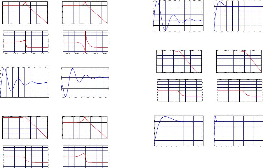
|
|
Exercises for Chapter 8 |
|
355 |
||
|
0 |
|
|
0 |
|
|
dB |
-20 |
|
dB |
-20 |
|
|
-40 |
|
-40 |
|
|
||
|
|
|
|
|
||
|
-60 |
|
|
-60 |
|
|
|
-3 -2 -1 0 |
1 |
2 3 4 |
|
-3 -2 -1 0 1 |
2 3 4 |
|
log ω |
|
|
|
log ω |
|
|
150 |
|
|
|
|
|
150 |
|
100 |
|
|
|
|
|
100 |
deg |
50 |
|
|
|
|
deg |
50 |
0 |
|
|
|
|
0 |
||
|
|
|
|
|
|
||
|
-50 |
|
|
|
|
|
-50 |
|
-100 |
|
|
|
|
|
-100 |
|
-150 |
|
|
|
|
|
-150 |
|
-3 -2 -1 |
0 |
1 |
2 |
3 |
4 |
|
log ω
-3 -2 -1 |
0 |
1 |
2 |
3 |
4 |
log ω
Bode plot 1 |
Bode plot 2 |
|
2 |
|
|
|
|
|
|
|
|
|
|
|
|
|
|
|
|
|
1.5 |
|
1.5 |
|
|
|
|
|
|
|
1 |
|
|
|
|
|
|
|
|
|
|
(t) |
1 |
|
|
|
|
|
|
(t) |
0.5 |
Σ |
|
|
|
|
|
|
Σ |
||
1 |
|
|
|
|
|
|
|
1 |
|
|
0.5 |
|
|
|
|
|
|
|
0 |
|
|
|
|
|
|
|
|
|
|
|
|
|
|
|
|
|
|
|
-0.5 |
|
0 |
|
|
|
|
|
|
|
|
|
2.5 |
5 |
7.5 |
10 |
12.5 |
15 |
17.5 |
20 |
|
|
|
|
|
t |
|
|
|
|
|
2.5 |
5 |
7.5 |
10 |
12.5 |
15 |
17.5 |
20 |
|
|
|
t |
|
|
|
|
Step response 1 |
|
Step response 2 |
(b) |
|
|
0 |
|
20 |
-20 |
|
0 |
|
|
|
dB-40 |
dB |
-20 |
|
||
-60 |
|
-40 |
|
|
|
|
|
-60 |
-3 -2 -1 0 1 2 3 4 |
|
-3 -2 -1 0 1 2 3 4 |
log ω |
|
log ω |
|
150 |
|
|
|
|
|
150 |
|
100 |
|
|
|
|
|
100 |
deg |
50 |
|
|
|
|
deg |
50 |
0 |
|
|
|
|
0 |
||
|
|
|
|
|
|
||
|
-50 |
|
|
|
|
|
-50 |
|
-100 |
|
|
|
|
|
-100 |
|
-150 |
|
|
|
|
|
-150 |
|
-3 -2 -1 |
0 |
1 |
2 |
3 |
4 |
|
log ω
-3 -2 -1 |
0 |
1 |
2 |
3 |
4 |
log ω
356 |
8 Performance of control systems |
22/10/2004 |
|
|
|
|
|
|
|
|
|
|
1.2 |
|
4 |
|
|
|
|
|
|
|
|
|
|
|
|
|
|
|
|
|
|
|
1 |
|
3 |
|
|
|
|
|
|
|
|
0.8 |
|
|
|
|
|
|
|
|
|
|
|
(t) |
2 |
|
|
|
|
|
|
|
(t) |
0.6 |
Σ |
|
|
|
|
|
|
|
|
Σ |
|
1 |
|
|
|
|
|
|
|
|
1 |
|
|
1 |
|
|
|
|
|
|
|
|
0.4 |
|
|
|
|
|
|
|
|
|
|
|
|
0 |
|
|
|
|
|
|
|
|
0.2 |
|
-1 |
2.5 |
5 |
7.5 |
10 |
12.5 |
15 |
17.5 |
20 |
0 |
|
|
|||||||||
|
|
|
||||||||
|
|
|
|
|
t |
|
|
|
|
|
2.5 |
5 |
7.5 |
10 |
12.5 |
15 |
17.5 |
20 |
|
|
|
t |
|
|
|
|
Step response 1 |
Step response 2 |
(c)
0 |
|
|
|
|
|
0 |
|
|
|
|
|
-10 |
|
|
|
|
|
-10 |
|
|
|
|
|
-20 |
|
|
|
|
|
-20 |
|
|
|
|
|
dB-30 |
|
|
|
|
|
dB-30 |
|
|
|
|
|
-40 |
|
|
|
|
|
-40 |
|
|
|
|
|
-50 |
|
|
|
|
|
-50 |
|
|
|
|
|
-3 -2 -1 |
0 |
1 |
2 |
3 |
4 |
-3 -2 -1 |
0 |
1 |
2 |
3 |
4 |
log ω |
log ω |
|
150 |
|
|
|
|
|
150 |
|
100 |
|
|
|
|
|
100 |
deg |
50 |
|
|
|
|
deg |
50 |
0 |
|
|
|
|
0 |
||
|
|
|
|
|
|
||
|
-50 |
|
|
|
|
|
-50 |
|
-100 |
|
|
|
|
|
-100 |
|
-150 |
|
|
|
|
|
-150 |
|
-3 -2 -1 |
0 |
1 |
2 |
3 |
4 |
|
log ω
-3 -2 -1 |
0 |
1 |
2 |
3 |
4 |
log ω
Bode plot 1 |
Bode plot 2 |
|
1.2 |
|
|
|
|
1.2 |
|
1 |
|
|
|
|
1 |
|
0.8 |
|
|
|
|
0.8 |
(t) |
0.6 |
|
|
|
(t) |
0.6 |
Σ |
|
|
|
Σ |
||
1 |
|
|
|
|
1 |
|
|
0.4 |
|
|
|
|
0.4 |
|
0.2 |
|
|
|
|
0.2 |
|
0 |
|
|
|
|
0 |
|
2 |
4 |
6 |
8 |
10 |
|
|
|
|
t |
|
|
|
2 |
4 |
6 |
8 |
10 |
|
|
t |
|
|
Step response 1 |
Step response 2 |
(d)
Bode plot 1 |
Bode plot 2 |