

диафрагмированные волноводные фильтры / 7ac4e4af-063a-4ed2-b8d5-43cf78ede2ce
.pdfDesign of Manifold-
Coupled Multiplexers
Richard J. Cameron and Ming Yu
Although the principles of combining or separating frequency diverse microwave signals (channels) for interfacing with a single port of an antenna system have been known for many years
now, it was with the advent of satellite communication systems in the 1970s that the greatest technical advances were made. In the satellite transponder itself, the uplinked channel groups from a common antenna need to be separated (demultiplexed) to allow separate routing and processing before power amplification and downlinking to (possibly) different zones on Earth (Figure 1). Here, very high selectivity is most critical to prevent adjacent channel interference and multipath effects. It is usually preferred that the bulk of the channel selectivity task as the channel passes through the transponder is done by the input demultiplexer (IMUX) filters to keep the output multiplexer (OMUX) filters as simple and low-loss as possible.
On the high-power side, the channels for downlinking need to be efficiently combined into one high-power composite output and transferred to the input port of an antenna feed system. Now, lowest possible loss is a priority, with a certain amount of selectivity to suppress out-of-band spectral regrowth caused by nonlinearities in the power amplifiers [traveling wave tube amplifiers (TWTAs) or solid-state power amplifiers (SSPAs)]. Further essential features that will be required of the IMUX and OMUX subsystems and their filters will be noted later.
Athird category of multiplexers that have been finding widespread application lately are the transmit/receive
© ARTVILLE
diplexers in the basestations of cellular telephony systems. These devices perhaps have the most demanding electrical and build-standard requirements of all, accommodating as they do both highand low-power signals in close proximity within one housing. In some cases, these diplexers are located at the top of transmitter masts, and there experience the worst of climatic extremes.
This article offers a brief overview of the principles of operation and the main design considerations for four different multiplexer subsystem configurations. The design method for the manifold multiplexer is
Richard J. Cameron and Ming Yu (ming.yu@ieee.org) are with COM DEV in Cambridge, Ontario, Canada.
Digital Object Identifier 10.1109/MMM.2007.904715
46 


 1527-3342/07/$25.00©2007 IEEE October 2007

explained in detail, using as an example the design and optimization of a four-channel output multiplexer. A more comprehensive review of waveguide (de)multiplexing systems—including practical information, design formulae, and a good bibliography—may be found in [1].
Multiplexer Configurations
Over the past three decades, there have been many advances in the design and implementation of multiplexing networks [1]–[23]. The most commonly used configurations are:
•hybrid-coupled multiplexers,
•circulator-coupled multiplexers,
•directional filter multiplexers, and
•manifold-coupled multiplexers.
High Power Amplifier
Low Noise |
MultiplexerInput |
MultiplexerOutput |
|
Receiver |
|||
|
|
||
Uplink |
|
Downlink |
|
|
Antenna |
||
Antenna |
|
||
|
|
Figure 1. A simplified block diagram of a satellite payload.
A summary of the advantages and disadvantages of these multiplexer configurations is given in Table 1 [6].
TABLE 1. A Comparison of Various Multiplexer Configurations.
Hybrid-Coupled |
Circulator- |
Directional |
Manifold |
Mux |
Coupled Mux |
Filter Mux |
Multiplexer |
Advantages |
Advantages |
Advantages |
Advantages |
|
|
|
|
–Amenable to a modular |
–Requires one filter per |
–Requires one filter |
–Requires one filter |
concept. |
channel. |
per channel. |
per channel. |
–Simple to tune, no |
–Employs standard |
–Simple to tune, no |
Most compact |
interaction between |
design of filters. |
interaction between |
design. |
channel filters. |
–Simple to tune. |
channel filters. |
|
|
–No interaction between |
|
|
|
channel filters. |
|
|
–Total power in |
–Amenable to a modular |
–Amenable to a |
–Capable of realizing |
transmission modes as |
concept. |
modular concept. |
optimum perfor- |
well as reflection mode is |
|
|
mance, both in terms |
divided by the hybrid so |
|
|
of absolute insertion |
that only 50% of the |
|
|
loss and amplitude |
power is incident on each |
|
|
and group delay |
filter. Power handling is |
|
|
response. |
thus increased and |
|
|
|
susceptibility to voltage |
|
|
|
breakdown is reduced. |
|
|
|
Disadvantages
–Two identical filters and two hybrids are required for each channel.
–Line lengths between hybrids and filters require precise balancing to preserve circuit directivity.
–The physical size and weight of the multiplexer is greater than other approaches.
Disadvantages |
Disadvantages |
Disadvantages |
–Signals must pass in |
–Restricted to realize |
–Complex design. |
succession through |
allpole functions such –Tuning of the |
|
circulators, incurring |
as Butterworth and |
multiplexer can be |
extra loss per trip. |
Chebyshev. |
time-consuming |
–Low-loss, high-power |
–Difficult to realize |
and expensive. |
ferrite circulators are |
bandwidths greater |
–Not amenable to a |
expensive. |
than 1%. |
flexible frequency |
|
|
plan, i.e., change of a |
–Higher level of passive |
–Restricted to the use |
channel frequency |
intermodulation (PIM) |
of single-mode filters. |
will require a new |
products than other |
|
multiplexer design. |
configurations. |
|
|
October 2007 |
47 |

f1,f2,...fn
f1 


f1 |
f2 |
f2 |
fn |
fn |
f1 |
|
f2 |
|
fn |
Figure 2. Layout of a hybrid-coupled multiplexer.
Hybrid-Coupled Approach
Figure 2 shows a layout of a hybrid-coupled multiplexer. Each channel consists of two identical filters and two identical 90◦ hybrids. The main advantage of the hybrid-coupled approach is its directional property, which minimizes the interaction between the channel filters. As a consequence, it is amenable to a modular concept, allowing the integration of additional channels at a later date without disrupting the existing multiplexer design, a requirement in some systems. Another key advantage of this approach is that only half of the input power goes through each filter. Thus, the filter design can be relaxed when using this type of multiplexer in high-power applications. On the other hand, it has the disadvantage of larger size since two filters and two hybrids per channel are required. Another design consideration of such multiplexers is the phase deviation between the two filter paths that the two signals undergo before they add constructively at the channel output. The structure, therefore, must be fabricated with tight tolerances to minimize the phase deviation.
f1,f2,...fn 
|
|
|
|
|
|
|
|
|
f1 |
|
f2 |
|
|
|
fn |
||
|
|
|||||||
Figure 3. A circulator-coupled multiplexer.
Circulator-Coupled Approach
Each channel in this case consists of a channel-dropping circulator and one filter, as shown in Figure 3. The unidirectional property of the circulator provides the same advantages as the hybrid-coupled approach in terms of amenability to modular integration and ease of design and assembly. The insertion loss of the first channel is the sum of the insertion loss of the channel filter and the insertion loss of the circulator. The subsequent channels exhibit a relatively higher loss due to the insertion loss incurred during each trip through the channel-dropping circulators. This is the most common realization for input multiplexers.
Directional Filter Approach
Figure 4 illustrates a layout of a multiplexer realized by connecting directional filters in series. A directional filter is a four-port device in which one port is terminated in a load. The other three ports of the directional filter essentially act as a circulator connected to a bandpass filter. Power incident at one port emerges at the second port with a bandpass frequency response while the reflected power from the filter emerges at the third port.
f1 |
f2 |
fn |
θ1 |
θ2 |
θn |
f1,f2,...fn
Figure 5. A manifold-coupled multiplexer.
|
|
f1 |
f2 |
f3 |
f4 |
|
|
|||||||||||||
|
|
|
|
|
||||||||||||||||
Input Signals |
|
|
Z1 |
|
|
Z2 |
|
|
Z3 |
|
|
Z4 |
|
|
||||||
|
|
|
|
|
|
|
|
|||||||||||||
|
|
a |
|
|
|
b |
|
|
|
c |
|
|
|
d |
|
|
|
|
||
|
|
|
|
|
|
|
|
|
|
|
|
|
||||||||
f1,f2,f3,f4,f5 |
|
|
|
|
|
|
|
|
|
|
|
|
|
|
|
|
|
|
|
f5 |
|
|
|
|
|
|
|
|
|
|
|
|
|
|
|
|
|
||||
|
|
|
|
|
|
|
|
|
|
|
|
|
|
|
|
|
|
|
|
|
Figure 4. A directional filter multiplexer.
48 |
October 2007 |

Directional filters, however, do not require the use of ferrite circulators. The waveguide version of a directional filter is typically realized by coupling rectangular waveguides operating in TE10 modes to a circular waveguide filter operating in TE11 modes. The microstrip version consists of one-wavelength ring resonators coupled to one another and to two transmission lines. This multiplexing approach has the same advantages as the hybrid-coupled and circulator-coupled approaches. It is, however, limited to narrow-band applications.
Manifold-Coupled Approach
The manifold-coupled approach shown in Figure 5 is viewed as the optimum choice as far as miniaturization and absolute insertion loss are concerned. This type of multiplexer requires the presence of all the channel filters at the same time so that the effect of channel interactions can be compensated in the design process. It implies that a manifold-coupled multiplexer is not amenable to a flexible frequency plan; any change in the allocation of channels will require a new multiplexer design. Moreover, as the number of channels increases, this approach becomes more difficult to implement. The manifold-coupled multiplexer shown in Figure 5 acts as a channelizer, but the same configuration can be used as a combiner. Figure 6 shows a 19-channel multiplexer employing a waveguide manifold. The manifold-cou- pled concept can be implemented as well in planar circuits as shown in Figure 7, where three high-tempera- ture superconductivity (HTS) microstrip filters are integrated with a microstrip manifold [17]. In this particular case, one of the channels is connected directly to the manifold. Figure 8 show a three-channel L-band multiplexer using coaxial manifold and combline channel filters. The manifold-coupled multiplexer is widely used for most OMUX applications today, and its design technique is the focus of this article.
Three common manifold multiplexer configurations are shown in Figure 9, with all channel filters connected to one side of the manifold (comb), to both sides (herringbone), and end-fed (applicable to either of the first two).
The technique is readily applicable to manifold multiplexers incorporating an arbitrary number of channels, regardless of their bandwidths and channel separations.
The design techniques for manifold multiplexers underwent rapid development in the 1970s and 1980s when it was realized that they were ideal for communication satellite payloads [4]–[7]. On the electrical side, design techniques have advanced to the point where it is possible to combine an arbitrary number of channels, regardless of their bandwidths and channel separations. There are no restrictions on the design and implementation of channel filters onto the manifold. The manifold itself is a transmission line, be it a coaxial line or a rectangular waveguide or some other low-loss structure. It is possible to achieve channel performance in the multiplexer configuration close to that of a channel filter by itself. No other multiplexer configuration can match this performance.
f1,f2,f3 |
|
|
f3 |
f1 |
f2 |
Figure 7. A three-channel planar HTS multiplexer [17].
Figure 6. A 19-channel Ku-band waveguide multiplexer [21].
Figure 8. A three-channel L-band multiplexer using coaxial manifold and combline channel filters [20].
October 2007 |
49 |

On the mechanical side, the entire structure may be made to be very lightweight and compact, while rugged enough to withstand the vibrations and other rigors of a launch into space. By using special materials, the whole structure may be made to be electrically stable in the presence of large environmental temperature fluctuations and be able to conduct dissipated RF thermal energy efficiently to a cooling baseplate [20].
Over the past three decades, there have been many advances in the design and implementation of multiplexing networks.
Design of the Manifold-Coupled Multiplexer
Design Methodology
Since there are no directional or isolating elements in the manifold multiplexer (circulators, hybrids), all channel filters are electrically connected to each other through the near lossless manifold and the design of the manifold multiplexer has to be considered as a whole, not as individual channels. In the early days, a number of ingenious techniques were invented [2]–[5], [8], [9] to design the individual filters such that they would properly interact with the other filters on the same manifold and function virtually as if they were operating into a matched termination. However, with the dramatic increase in computer power that has become available in recent years, practical multiplexer
design procedure has tended to utilize optimization methods to achieve the final design, in preference to the more limited analytic techniques.
Analysis of Common-Port Return Loss and Channel Transfer Characteristics
At the heart of any circuit optimizer is an efficient analysis routine, for the optimization will call the analysis routine many thousands of times at different frequencies as it progresses with the task of optimizing the various parameters [11]. In general, the two parameters from which the overall cost function is built up are the multiplexer common-port return loss (CPRL) and the individual channel transfer characteristics.
During the optimization process, the subroutines to calculate CPRL channel transfer characteristics at each frequency sampling point will be called many times. Although it would be possible to construct an admittance matrix for the whole multiplexer circuit and analyze it at each frequency point to obtain the desired transfer and reflection data, this matrix will be quite large for the multiplexer with a large number of channel filters and will take a significant amount of CPU time to invert it even though it will be relatively sparse. Moreover, a lot of data will be obtained that is not used for the optimization.
Later on in this section a piecewise optimization strategy, which has been found to be quite efficient in terms of computer CPU time, will be described [13], [14]. Part of the strategy involves optimizing the channel filters one after the other in a repeated cycle. As the optimization parameters of each filter in turn are being optimized, it is only necessary to calculate the transfer
|
|
|
|
|
Channel 1 |
Channel |
Channel |
|
|
|
1 |
|
|
|
Channel |
||
Channel 1 |
|
|
|
||
Channel 1 |
|
|
|
||
Inputs |
Filters |
Short |
|
|
|
|
|
|
|
||
|
|
Manifold |
|
|
|
Channel 2 |
Channel 2 |
Channel 1 |
Channel 1 |
Channel 2 |
Channel 2 |
|
|
|
|
||
Channel 3 |
Channel 3 |
|
Channel 2 |
Channel 2 |
|
Channel 3 |
Channel 3 |
Channel 3 |
Channel 3 |
||
|
|
|
|
||
Channel 4 |
Channel 4 |
|
Channel 4 |
Channel 4 |
|
Channel 5 |
Channel 5 |
Channel 4 |
Channel 4 |
||
|
|
|
|
||
Channel 5 |
Channel 5 |
|
Common Port |
Channel 5 |
Channel 5 |
|
Output |
||||
|
|
|
|
|
|
|
Common Port |
|
|
Common Port |
|
|
Output |
|
|
||
|
|
|
Output |
||
|
|
|
|
|
|
|
(a) |
|
(b) |
|
(c) |
Figure 9. Common configurations for manifold multiplexers: (a) comb, (b) herringbone, and (c) one filter feeding directly into the manifold.
50 |
October 2007 |

characteristic of this |
filter |
|
|
|
|
|
|
|
|
|
|
|
|
|
|
|
|
|
|||
alone; the others will be rela- |
|
|
|
|
|
|
|
|
|
Terminating |
|
|
|
||||||||
tively |
unaffected |
by the |
|
|
|
|
|
|
|
|
|
Impedance (=1Ω) |
|
|
|
||||||
changes (assumed |
small) |
|
|
|
|
|
|
|
|
|
|
|
|
|
|
|
|
|
|||
being made to the filter that |
|
|
|
|
|
|
|
|
|
|
|
|
|
|
|
|
|
||||
|
|
|
|
|
|
|
|
|
|
|
|
|
|
|
|
|
|||||
is the object of the optimiz- |
|
|
|
|
|
|
|
|
|
|
|
|
|
|
|
|
|
||||
er’s attentions at this stage in |
|
|
Channel 3 |
|
|
|
Channel 2 |
|
|
|
Channel 1 |
|
|
|
|
|
|||||
the cycle. |
|
|
|
|
|
|
|
|
|
|
|
|
|
|
|
|
|||||
|
|
|
|
|
Filter |
|
|
|
Filter |
|
|
|
|
Filter |
|
|
|
|
|
||
To speed up the overall |
|
|
|
|
|
|
|
|
|
|
|
|
|
|
|||||||
|
|
|
|
|
|
|
|
|
|
|
|
|
|
|
|
|
|||||
optimization, |
it |
becomes |
|
|
|
|
|
|
|
|
|
|
|
|
|
Stub |
|
||||
more |
efficient |
to |
analyze |
|
|
|
|
|
|
|
|
|
|
|
|
|
≈ |
nλ |
|
||
|
|
|
|
|
|
|
|
|
|
|
|
|
|
||||||||
each filter’s input-to-com- |
|
|
|
|
|
|
|
|
|
|
|
|
|
2 |
|
|
|||||
|
|
|
|
|
|
|
|
|
|
|
|
|
|
|
|
||||||
|
|
|
|
|
|
|
|
|
|
|
|
|
|
|
|
||||||
mon-port transfer character- |
|
|
|
|
|
|
|
|
|
|
|
|
|
|
|
|
|
||||
|
|
|
|
|
|
|
|
|
|
|
|
|
|
|
|
|
|||||
istic individually, in addition |
|
Common |
J3 |
|
|
|
J2 |
|
|
|
|
J1 |
|
|
|
|
Short |
||||
|
|
|
|
|
|
|
|
|
|
|
|
||||||||||
to the CPRL. The manifold of |
|
Port |
|
|
|
|
|
|
|
|
|
|
|
Circuit |
|||||||
|
|
|
|
|
|
|
|
|
|
|
|
|
|
|
|||||||
the multiplexer may be most |
|
|
|
|
|
|
|
|
|
|
|
|
|
|
|
|
|
||||
|
|
|
|
|
|
|
|
|
|
|
|
|
|
|
|
|
|||||
conveniently represented as |
|
|
Interjunction Spacings |
≈ |
nλ |
|
|
Waveguide |
|
|
|
||||||||||
|
|
|
|
|
|
|
|||||||||||||||
an open-wire circuit, with a |
|
|
|
|
|
|
|
||||||||||||||
|
|
|
|
|
|
|
|
||||||||||||||
short circuit at one end and |
|
|
|
|
|
|
|
2 |
|
|
Junction |
|
|
|
|||||||
|
|
|
|
|
|
|
|
|
|
|
|
|
|
||||||||
|
|
|
|
|
|
|
|
|
|
|
|
|
|
|
|
|
|||||
three-port junctions spaced |
|
|
|
|
|
|
|
|
|
|
|
|
|
|
|
|
|
||||
Figure 10. Open-wire model of waveguide manifold multiplexer (three-channel). |
|
||||||||||||||||||||
along its length. The channel |
|
||||||||||||||||||||
filters are located at the third |
|
|
|
|
|
|
|
|
|
|
|
|
|
|
|
|
|
||||
port of each junction and are |
|
|
|
|
|
|
|
|
|
|
|
|
|
|
|
|
|
||||
separated from the junction by short lengths of trans- |
ing the possibility for port 3 to be a different size as |
mission lines (stubs) as shown in Figure 10. |
described in Figure 11. |
If the manifold is waveguide, the junctions may be |
Because of reciprocity and the symmetry of the junc- |
E-plane or H-plane, and since their intrinsic parame- |
tions about the vertical axis in Figure 11, S22 = S11 and |
ters do not change during the optimization, they are |
S32 = S31 (H-plane) and S32 = −S31 (E-plane). This |
best characterized with three-port S-parameters pre- |
means that only four parameters—S11, S21, S31, and |
calculated by a mode-matching routine and stored |
S33—are needed to completely characterize the electri- |
over a range of frequencies covering the bandwidths |
cal performance of the junctions. The S-parameter |
of all the channel filters, or specifically at the frequen- |
matrices are calculated assuming a matched termina- |
cies of the sampling points. Coaxial junctions are a spe- |
tion at each port, but if the termination at one port is |
cial case of waveguide junction (H-plane). Typically, |
arbitrary, the two-port S-parameters between the other |
the junctions are symmetric about ports 1 and 2, leav- |
two ports may be defined as follows. |
|
|
|
|
|
|
|
|
|
|
|
|
|
|
|
|
|
Plane of |
|
|
Plane of |
|
|
|
|
|||||||||||||||||
|
|
|
|
|
|
Y3=1 |
|
|
|
|
|
|
Symmetry |
|
|
Symmetry |
|||||||||||||||||||||||||
|
|
|
|
|
|
|
|
|
|
|
|
|
|
|
|
|
|
|
|
|
|
|
|
|
|
|
|
|
|
|
|
|
|
|
|
|
|||||
|
|
|
|
|
|
|
|
|
|
|
|
|
|
|
|
|
|
|
a1 |
|
|
|
|
|
|
|
|
|
|
|
|
|
|
|
|
|
|
|
|
|
|
|
|
|
|
|
|
|
|
|
|
|
|
|
|
|
|
|
|
|
|
|
|
|
|
|
|
|
|
|
|
|
|
|
|
|
|
|
|
|
|
||
|
|
|
|
|
|
|
|
|
|
|
|
|
|
|
|
|
|
|
|
|
|
|
|
|
|
|
|
|
|
|
|
|
|
|
|
|
|
|
|
||
|
|
|
|
|
|
|
|
|
|
|
|
|
|
|
|
|
|
3 |
|
|
|
|
|
|
|
|
|
|
|
|
|
b1 |
|
|
|
|
|
||||
|
|
|
|
|
|
3 |
|
|
|
|
|
|
|
|
|
|
|
|
|
|
|
|
|
|
|
|
|
|
|
|
|
|
3 |
|
|
|
|
|
|
||
|
|
|
|
|
|
|
|
|
|
|
|
|
|
1 |
|
|
|
|
|
|
2 |
|
|
|
|
|
|
|
|
|
|
|
|
|
|
|
|||||
|
|
|
|
|
|
|
|
|
|
|
|
|
|
|
|
|
|
|
|
|
|
|
|
|
|
|
|
|
|
|
|
|
|
|
|
||||||
Y1=1 |
|
|
|
|
1 |
2 |
|
|
|
|
Y2=1 |
a |
|
|
|
|
|
a |
|
|
|
|
|
|
|
|
|
|
|
|
|
|
|
|
|||||||
|
|
|
|
|
|
|
|
|
|
b |
|
1 |
|
|
|
|
|
|
|
2 b |
|
|
|||||||||||||||||||
|
|
|
|
|
|
|
|
|
|
|
|
|
|
|
|
|
|
||||||||||||||||||||||||
|
|
|
|
|
|
|
|
|
|
|
|
|
|
|
|
|
|
|
|
|
|
|
|
|
|
|
|
|
|
|
|
|
|
|
|
|
|||||
|
|
|
|
|
|
|
|
|
|
|
|
|
|
|
|
|
|
|
|
|
|
|
|
|
|
|
|
|
|
|
|
|
|
|
|
|
|
|
|
|
|
|
|
|
|
|
|
|
|
|
|
|
|
|
|
|
|
|
|
|
|
|
|
|
E-Plane |
|
|
|
|
||||||||||||||
|
|
|
E-Plane or H-Plane |
|
|
|
|
|
|
H-Plane |
|
|
|
|
|
|
|||||||||||||||||||||||||
|
|
|
|
|
Junction |
|
|
|
|
|
|
Junction |
|
|
Junction |
|
|
|
|
||||||||||||||||||||||
|
|
|
|
S11 S12 S13 |
|
|
|
|
|
|
S11 S21 S31 |
|
|
|
S11 |
|
|
S21 |
S31 |
|
|||||||||||||||||||||
|
|
|
|
S21 S22 S23 |
|
|
|
|
|
|
S21 S11 S31 |
|
|
|
S21 |
|
|
S11 |
−S31 |
|
|||||||||||||||||||||
|
|
|
|
S31 |
S32 S33 |
|
|
|
|
|
|
S31 S31 |
S33 |
|
|
|
S31 |
|
|
−S31 |
S33 |
|
|||||||||||||||||||
|
|
|
|
|
|
|
|
|
|
|
|
|
|
|
|
|
|
|
|
|
|
|
|
|
|
|
|
|
|
|
|
|
|
|
|
|
|
|
|
|
|
Figure 11. E-plane and H-plane waveguide junctions and S-parameter matrix representation.
October 2007 |
51 |

|
|
|
|
|
|
|
|
|
|
|
|
|
|
|
|
|
|
|
|
|
|
|
|
|
|
|
|
|
|
|
|
|
|
|
Channel 3 |
Filter |
|
|
Channel 2 |
Filter |
|
Channel 1 |
Filter |
||||
|
YF3 |
YF2 |
YF1 |
|
J3 |
J2 |
J1 |
YM4 |
YM3 |
YM 2 |
YM1 |
Figure 12. CPRL computation.
YF 3 |
Channel 2 |
Filter |
YF1 |
|
|
||
|
|
YF 2 |
|
J3 |
J2 |
J1 |
|
|
|
YM 2 |
|
Figure 13. Channel 2 transfer function calculation.
1) Admittance YL2(= 1) at port 2:
S11 |
S13 |
S11 |
S13 |
|
|
|
S31 |
S33 = |
S31 |
S33 |
|
|
|
|
2 |
S212 |
|
kS21S31 |
|
|
+ |
|
kS21S31 |
S312 |
, |
(1) |
|
1 − 2S11 |
||||||
where 2 = (1 − YL2)/(1 + YL2), YL2 is the admittance at port 2 of the junction, and k = 1 for H-plane junctions and -1 for E-plane junctions. This modified S–matrix also applies if an admittance YL1 is terminating port 1. It is only necessary to change the subscripts from 2 to 1 and vice versa.
2) Admittance YL3(= 1) at port 3:
S11 |
S12 |
= |
S11 |
|
S12 |
|
||
S21 |
S22 |
S21 |
|
S22 |
||||
|
|
3S2 |
1 |
k |
|
|
||
+ |
|
|
|
31 |
k |
1 |
, |
(2) |
|
− |
|
3S33 |
|||||
1 |
|
|
|
|
|
|||
where 3 = (1 − YL3)/(1 + YL3), YL3 is the admittance at port 3 of the junction, and k has the same meaning as before. These junction S-parameters may be easily converted to the [ABCD] transfer parameters using standard formulas to enable cascading with the channel filters and stub/manifold line lengths.
CPRL
The common port return loss (CPRL) computation at a given frequency point (e.g., at a sample point) proceeds as follows:
1)Determine the channel filter input admittances YF1, YF2, and YF3 at the frequency sample point and store (see Figure 12).
2)Now with known admittances at the port 3 of each
junction, the transfer and reflection S-parameters [S21, S11, see (2)] for each junction may be calculated and converted to [ABCD] matrices. Now working
from the short-circuit end, the manifold phase lengths and the junctions may be cascaded, at each stage calculating and storing the along-manifold admittances YM1, YM 2, etc. as shown in Figure 12.
YMi = |
1 |
+ S11i |
, |
( ) |
|
1 |
− S11i |
||||
|
3 |
where i = 1, 2, . . . n + 1 and n is the number of channels on the manifold.
The final admittance (YM4 in Figure 12) may be used to calculate the CPRL
|
1 + YMn+1 |
|
CP = |
1 − YMn+1 |
|
RLCP = −20 log10 CP (dB) |
(4) |
|
If only the manifold spacings θM1, θM2, . . . are being optimized, then the filter input admittances YF1, YF2, . . .
etc. need only be calculated once at each sample frequency and stored for the optimization of CPRL.
Channel Transfer Characteristics
If optimization is now focused on an individual channel filter and the transfer function between its input and the common port is needed (e.g., for a rejection sample point), the following procedure may be used:
Taking channel 2 as an example, as shown in Figure 13,
1)Calculate the new YF2 for channel 2 with its newly updated parameters.
2)The previously stored value of YM2 may be used in conjunction with equation (1) to calculate S31 and S11 for junction 2 with YM2 at its port 2.
3)The [ABCD] matrices for the channel 2 filter and the S31 path of J2, and then the rest of the manifold towards the common port (the manifold line length between J2 and J3, then using equation (2) to find the [ABCD] parameters of J3 terminated with YF3 at its port 3) may then be cascaded to calculate the
transfer characteristic for channel 2. The process may be repeated for the other channels.
For both common-port and transfer characteristics, the computations may be made assuming lossless (purely reactive) components for the filter and stub networks. Then noncomplex arithmetic may be used for the matrix multiplications, inversions, and other calculations, and the process is considerably speeded up.
52 |
October 2007 |

Channel Filter Design
Being purely reactive (i.e., no resis- |
|
1.5 |
|
|
|
|
|
|
|
|
|
|
|
|||
tive elements between the channel |
|
|
Imaginary |
|
|
|
|
|
|
|
|
|
||||
inputs and the common-port out- |
(MHOS) |
1 |
|
Part |
|
|
|
|
|
|
Real Part |
|
||||
put), the channel filters of the mani- |
|
|
|
|
|
|
|
|
|
|
||||||
fold multiplexer will react with each |
0.5 |
|
|
|
|
|
|
|
|
|
|
|
||||
other through the manifold itself. If |
Admittance |
|
|
|
|
|
|
|
|
|
|
|
||||
|
|
|
|
|
|
|
|
|
|
|
|
|||||
the channels are widely spaced, the |
|
|
|
|
|
|
|
|
|
|
|
|
||||
channel |
interactions are |
quite low, |
0 |
|
|
|
|
|
|
|
|
|
|
|
||
because |
over one filter’s |
passband |
|
|
|
|
|
|
|
|
|
|
|
|
||
Input −0.5 |
|
Complex Input Admittance |
|
|
|
|
|
|
||||||||
the other filters are well into their |
|
|
|
|
|
|
|
|||||||||
|
of Singly - Terminated Filter |
|
|
|
|
|
|
|||||||||
reject regions and will be presenting |
|
|
|
(6th Degree Quasi - Elliptic) |
|
|
|
|
|
|
||||||
short circuits at their ports nearest to |
|
−1 |
|
|
|
|
|
|
|
|
|
|
|
|||
the manifold. The channel filters |
|
−2.5 |
−2 |
−1.5 |
−1 |
−0.5 |
0 |
0.5 |
1 |
1.5 |
2 |
2.5 |
||||
may be designed as doubly terminat- |
|
|
|
|
|
|
Freq (rad/s) |
|
|
|
|
|||||
ed networks separate from the other |
|
|
|
|
|
|
|
(a) |
|
|
|
|
|
|||
filters and the manifold and, when |
|
1.5 |
|
|
|
|
|
|
|
|
|
|
|
|||
integrated onto the manifold, all that |
|
|
|
|
|
|
|
|
|
|
|
|
||||
|
|
|
|
|
|
|
|
|
|
|
|
|
||||
is needed are adjustments to the |
(MHOS) |
1 |
|
|
|
|
|
|
|
|
|
|
||||
along-manifold spacings and stub |
Real Part |
|
|
|
|
|
|
|
|
|||||||
|
|
|
|
|
|
|
|
|
|
|||||||
lengths |
and minor adjustments to |
|
|
|
|
|
|
|
|
|
|
|
|
|||
the first three or four elements of the |
0.5 |
|
|
|
|
|
|
|
|
|
|
|
||||
Admittance |
|
|
|
|
|
|
|
|
Imaginary |
|
||||||
filter to recover a good CPRL. |
|
|
|
|
|
|
|
|
|
|
||||||
|
|
|
|
|
|
|
|
|
|
Part |
|
|||||
However, as the guard bands |
0 |
|
|
|
|
|
|
|
|
|
|
|
||||
between channel filters |
decrease |
|
|
|
|
|
|
|
|
|
|
|
|
|||
Input |
|
|
|
|
|
|
|
|
|
|
|
|
||||
towards contiguity, they begin to |
−0.5 |
|
|
|
Complex Input Admittance |
|
|
|
|
|||||||
interact strongly along the mani- |
|
|
|
|
|
of Doubly - Terminated Filter |
|
|
|
|
||||||
fold. Now significant adjustments |
|
−1 |
|
|
(6th Degree Quasi - Elliptic) |
|
|
|
|
|||||||
to the filter parameters are needed |
|
−2 |
−1.5 |
−1 |
−0.5 |
0 |
0.5 |
1 |
1.5 |
2 |
2.5 |
|||||
|
−2.5 |
|||||||||||||||
in addition to the manifold and stub |
|
|
|
|
|
|
Freq (rad/s) |
|
|
|
|
|||||
phase lengths to reach an acceptable |
|
|
|
|
|
|
|
(b) |
|
|
|
|
|
|||
CPRL. Although it is possible to |
Figure 14. Characteristics of the real and imaginary parts of prototype input |
|||||||||||||||
optimize doubly terminated filters |
||||||||||||||||
to operate in a contiguous channel |
admittance: (a) singly terminated filter and (b) doubly terminated filter. |
|
||||||||||||||
environment, a starting point much |
|
|
|
|
|
|
|
|
|
|
|
|
|
|||
closer to the final optimal result is |
|
2 |
|
|
|
|
|
|
|
|
|
|
|
|||
obtained if singly terminated filter |
|
|
|
|
|
|
|
|
|
|
|
|
||||
|
|
|
|
|
|
|
|
|
|
|
|
|
||||
prototypes are used in these condi- |
(MHOS) |
|
|
|
|
|
|
|
|
|
|
Real Part |
||||
tions. The design methods for singly |
1 |
|
|
|
|
|
|
|
|
|
|
|
||||
terminated filter prototypes are out- |
|
|
|
|
|
|
|
|
|
|
|
|||||
|
|
|
|
|
|
|
|
|
|
|
|
|||||
Admittance |
|
|
|
|
|
|
|
|
|
|
|
|
||||
lined in [2] and [18]. |
|
|
|
|
|
|
|
|
|
fo3 |
|
|
|
|||
The singly terminated |
filter net- |
|
|
|
|
|
|
|
|
|
|
|
||||
0 |
|
|
|
|
|
|
|
|
|
|
|
|||||
work is useful for the design of con- |
|
|
|
|
|
|
|
|
|
|
|
|||||
|
|
|
|
fo1 |
|
fo2 |
|
|
|
|
|
|||||
tiguous channel manifold multiplexers |
|
|
|
|
|
|
|
|
|
|
||||||
Composite |
|
|
|
|
|
|
|
|
|
|
||||||
|
|
|
|
|
|
|
|
|
|
|
|
|||||
because the contiguous singly termi- |
−1 |
Composite Admittance - |
|
|
Imaginary Part |
|
|
|||||||||
nated channel filters along the mani- |
|
3 - Channel Contiguous |
|
|
|
|
||||||||||
|
|
|
|
|
|
|
|
|||||||||
fold tend to interact in a mutually ben- |
|
|
Multiplexer |
|
|
|
|
|
|
|
|
|||||
|
|
|
|
|
|
|
|
|
|
|
|
|
||||
eficial manner, providing a conjugate |
|
−2 |
|
−4 |
−3 |
−2 |
−1 |
0 |
1 |
2 |
3 |
4 |
5 |
|||
match for each other at their launch |
|
−5 |
|
|||||||||||||
|
|
|
|
|
|
Freq (rad/s) |
|
|
|
|
||||||
points. This natural multiplexing effect |
|
|
|
|
|
|
|
|
|
|
||||||
|
|
|
|
|
|
|
|
|
|
|
|
|
||||
may be explained by studying the spe- |
Figure 15. Singly terminated filter at center frequency f02 with two contiguous |
|||||||||||||||
cial characteristics of the input admit- |
||||||||||||||||
neighbors f01 and f03. Composite admittances as seen from the common port of |
||||||||||||||||
tance of the singly terminated circuit |
the manifold. |
|
|
|
|
|
|
|
|
|
||||||
looking in at the port opposite to the |
|
|
|
|
|
|
|
|
|
|
|
|
|
|||
terminated port (YF1, YF2, . . . etc. in Figure 12). |
|
|
teristic. It is close to unity over the filter’s passband, |
|||||||||||||
The real part of the input admittance has the same |
dropping to near zero in the out-of-band regions. As fre- |
|||||||||||||||
characteristic as the filter’s own power transfer charac- |
quency increases from minus infinity, the imaginary part |
|||||||||||||||
October 2007 |
53 |

|
0 |
|
|
|
|
|
|
|
|
real part of the source most- |
||
|
|
|
|
|
|
|
|
|
ly sees the unity load at the |
|||
|
|
|
|
|
|
|
|
|
|
|||
|
|
|
|
|
|
|
|
4-Channel |
|
common port of the mani- |
||
|
|
|
|
|
|
|
Contiguous MUX - |
fold, the impedances at the |
||||
|
|
|
|
|
|
|
|
Superimposed |
|
|||
|
10 |
|
|
|
|
|
|
|
input |
ports |
of the other |
|
|
|
|
|
|
|
Channel Rejections |
||||||
|
|
|
|
|
|
|
|
Preoptimization |
|
channel filters being mostly |
||
(dB) |
|
|
|
|
|
|
|
Performance |
|
|||
|
|
|
|
|
|
|
|
isolated by their own rejec- |
||||
|
|
|
|
|
|
|
|
|
||||
Rejection |
|
|
|
|
|
|
|
|
|
between the source and the |
||
|
20 |
|
|
|
|
|
|
|
|
tion characteristics. |
||
|
|
|
|
|
|
|
|
|
Thus, a conjugate match |
|||
|
|
|
|
|
|
|
|
|
|
|||
|
30 |
|
|
|
|
|
|
|
|
load |
has been partially |
|
|
|
|
|
|
|
|
|
|
achieved for channel filter |
|||
|
|
|
|
|
|
|
|
|
|
|||
|
|
|
|
|
|
|
|
|
|
f02. Although it will not be |
||
|
|
|
|
|
|
|
|
|
|
a perfect conjugate match, |
||
|
40 |
12,500 |
12,550 |
12,600 |
12,650 |
12,700 |
12,750 |
12,800 |
12,850 |
it will be better than if dou- |
||
|
12,450 |
bly terminated filters had |
||||||||||
|
|
|
|
Frequency (MHz) |
|
|
|
|||||
|
|
|
|
|
|
|
been used, and it makes a |
|||||
|
|
|
|
|
|
|
|
|
|
|||
|
|
|
|
|
(a) |
|
|
|
|
good point from which to |
||
|
0 |
|
|
|
|
|
|
|
|
start |
the |
optimization |
|
|
|
|
|
|
|
|
|
process. The channels f01 |
|||
|
|
|
|
|
|
|
|
|
|
|||
(dB) |
|
|
|
|
|
|
|
|
|
and f03 at the edges of the |
||
10 |
|
|
|
|
|
|
|
|
contiguous |
group on the |
||
Loss |
|
|
|
|
|
|
|
|
manifold, having a neigh- |
|||
|
|
|
|
|
|
|
|
|
||||
|
|
|
|
|
|
|
|
|
|
|||
Return |
20 |
|
|
|
|
|
|
|
|
bor on one side only, will |
||
|
|
|
|
|
|
|
|
tend to have some small in- |
||||
|
|
|
|
|
|
|
|
|
|
|||
Port |
|
|
|
|
|
|
|
|
|
band and rejection asym- |
||
|
|
|
|
|
|
|
|
|
metries after the optimiza- |
|||
|
|
|
|
|
|
|
|
|
|
|||
Common |
|
|
|
|
|
|
|
|
|
tion process. |
|
|
30 |
|
|
|
|
4 - Channel Contiguous MUX - |
|
|
|
||||
|
|
|
|
|
|
Common Port Return Loss |
|
Optimization Strategy |
||||
|
|
|
|
|
|
Preoptimization Performance |
||||||
|
|
|
|
|
|
|
|
|
|
|
|
|
The networks that model |
40 |
|
|
|
|
|
|
|
|
|
|
|
|
even a moderate-sized wave- |
|
|
|
|
|
|
|
|
|
|
|
|
guide manifold multiplexer |
|
12,500 |
12,550 |
12,600 |
12,650 |
12,700 |
12,750 |
12,800 |
|||||||
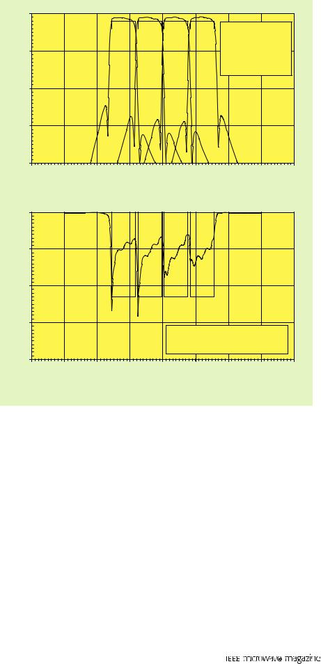
tend to be quite complex. An open-wire equivalent circuit of a six-channel manifold multiplexer with sixth-degree quasi-elliptic dual-mode filters has in
the order of 90 frequency sampling points and 100 electrical elements of varying sensitivities and different constraints that all need to be correctly valued before the overall multiplexer will operate to specification.
If all these parameters are optimized simultaneously, not only will the amount of CPU time be enormous, but there is little likelihood that the global optimum will be attained, there being a myriad of shallow local optimum solutions. With manifold multiplexers routinely incorporating 20 channels, and perhaps up to 30 in the future, global optimization is clearly unsuitable directly from the start.
For these reasons, most of the major satellite OMUX designers and manufacturers have developed more efficient methods for manifold multiplexer optimization. Among these is the piecewise approach, optimizing parts of the multiplexer separately in repeated cycles while converging upon an optimal solution. The parts or
54 |
October 2007 |
parameter |
|
groups |
being |
|
0 |
|
|
|
|
|
|
|
|
||||
referred |
to |
here |
might |
|
|
|
|
|
|
|
|
|
|||||
|
|
|
|
|
|
|
|
|
|
||||||||
include the first five elements |
|
|
|
|
|
|
|
4 - Channel Contiguous |
|||||||||
of |
each channel filter (nar- |
|
|
|
|
|
|
|
|
MUX |
|
||||||
row-band domain), or all the |
|
10 |
|
|
|
|
|
Superimposed Channel |
|||||||||
|
|
|
|
|
|
|
Rejections |
|
|||||||||
manifold |
interjunction |
or |
(dB) |
|
|
|
|
|
|
After Optimization of |
|||||||
stub |
lengths |
(wideband |
|
|
|
|
|
|
Manifold Spacings |
||||||||
|
|
|
|
|
|
|
|
|
|||||||||
domain). It is usual practice |
|
|
|
|
|
|
|
|
|
||||||||
Rejection |
20 |
|
|
|
|
|
|
|
|
||||||||
to commence the optimiza- |
|
|
|
|
|
|
|
|
|||||||||
|
|
|
|
|
|
|
|
|
|||||||||
tion process with the wide- |
|
|
|
|
|
|
|
|
|
||||||||
band sections first (parame- |
|
|
|
|
|
|
|
|
|
||||||||
|
30 |
|
|
|
|
|
|
|
|
||||||||
ters relating to the manifold |
|
|
|
|
|
|
|
|
|
||||||||
and stubs), followed by a |
|
|
|
|
|
|
|
|
|
|
|||||||
shift in emphasis to the nar- |
|
|
|
|
|
|
|
|
|
|
|||||||
row-band sections (filter |
|
40 |
|
|
|
|
|
|
|
|
|||||||
parameters) |
as |
the |
CPRL |
|
12,450 |
12,500 |
12,550 |
12,600 12,650 12,700 12,750 12,800 12,850 |
|||||||||
begins to take shape. A typi- |
|
|
|
|
Frequency (MHz) |
|
|
|
|||||||||
cal design optimization pro- |
|
|
|
|
|
(a) |
|
|
|
|
|||||||
ject might proceed as follows: |
|
0 |
|
|
|
|
|
|
|
|
|||||||
• Design |
|
|
|
|
|
|
|
|
|
|
|
|
|
|
|||
|
|
|
|
|
|
|
|
|
|
|
|
|
|
|
|||
1) |
Design the channel filter |
(dB) |
|
|
|
|
|
|
|
|
|
||||||
|
transfer/reflection func- |
|
|
|
|
|
|
|
|
|
|||||||
|
tions to meet the individ- |
10 |
|
|
|
|
|
|
|
|
|||||||
|
Loss |
|
|
|
|
|
|
|
|
||||||||
|
ual in-band and rejection |
|
|
|
|
|
|
|
|
|
|||||||
|
specifications. |
|
|
Return |
|
|
|
|
|
|
|
|
|
||||
2) |
Synthesize |
the |
corre- |
20 |
|
|
|
|
|
|
|
|
|||||
|
sponding coupling matri- |
Port |
|
|
|
|
|
|
|
|
|
||||||
|
ces, doubly terminated if |
|
|
|
|
|
|
|
|
|
|||||||
|
Common |
|
|
|
|
|
|
|
|
|
|||||||
|
the |
channel |
filter |
design |
30 |
|
|
|
|
|
|
|
|
||||
|
bandwidths |
(DBWs) |
are |
|
|
|
|
|
|
|
|
||||||
|
|
|
|
|
|
4 - Channel Contiguous MUX - |
|
||||||||||
|
separated by guard bands |
|
|
|
|
|
|
||||||||||
|
|
|
|
|
|
Common Port Return Loss |
|
||||||||||
|
|
|
|
|
|
|
|
||||||||||
|
greater than about 25% of |
|
|
|
|
|
After Optimization of Manifold Spacings |
||||||||||
|
|
40 |
|
|
|
|
|
|
|
|
|||||||
|
the DBWs, singly termi- |
|
12,500 |
12,550 |
12,600 |
12,650 |
12,700 |
12,750 |
12,800 |
12,850 |
|||||||
|
nated |
if |
otherwise. |
If |
|
12,450 |
|||||||||||
|
|
|
|
|
Frequency (MHz) |
|
|
|
|||||||||
|
singly terminated |
proto- |
|
|
|
|
|
|
|
||||||||
|
|
|
|
|
|
(b) |
|
|
|
|
|||||||
|
types are to be used, a |
|
|
|
|
|
|
|
|
|
|||||||
|
more |
practical |
design |
Figure 17. Four-channel manifold multiplexer after optimization of manifold lengths: |
|||||||||||||
|
results if the initial pro- |
||||||||||||||||
|
(a) superimposed channel transfer characteristics and (b) CPRL. |
|
|
|
|||||||||||||
|
totype is generated with |
|
|
|
|||||||||||||
|
|
|
|
|
|
|
|
|
|
|
|||||||
|
a low return loss to bring |
|
|
|
|
|
|
|
|
|
|
||||||
|
the value of the termination at the end opposite to |
2) Optimize stubs and the first three or four parame- |
|||||||||||||||
|
the manifold as close to unity as possible. |
|
ters of channel filter 1 [MS1 (filter manifold cou- |
||||||||||||||
3. |
Set initial manifold spacings between E- or H-plane |
pling), M11 (first resonance tuning), and M12 (reso- |
|||||||||||||||
|
junctions at mλg/2, where m is as low as possible for |
nance 1 to resonance 2 coupling)]. |
|
||||||||||||||
|
a convenient mechanical layout. Set the initial man- |
3) Repeat the cycle for all the channels, possibly |
|||||||||||||||
|
ifold short/first junction spacing at λg/4 (H-plane) |
omitting the stub length since this does not |
|||||||||||||||
|
or λg/2 (E-plane). λg is the wavelength in the mani- |
change much after the first cycle of optimization, |
|||||||||||||||
|
fold waveguide at the center frequency of the near- |
until the improvements in the cost function begin |
|||||||||||||||
|
est filter to the length of waveguide in the direction |
to become negligible. |
|
|
|
||||||||||||
|
of the common port. |
|
|
|
|
|
• Refinement |
|
|
|
|
||||||
4. |
Set initial manifold junction-filter stub lengths at |
1) Repeat optimization of manifold and stub lengths. |
|||||||||||||||
|
nλg/2. Again, n should be as small as possible. |
|
2) Reoptimization with a fine step on all of each chan- |
||||||||||||||
• Optimization |
|
|
|
|
|
|
|
nel filter’s parameters, most lightly on the ele- |
|||||||||
1) |
Design wideband components. Optimize spacings |
ments furthest away from the manifold, and not at |
|||||||||||||||
|
between the junctions and between the short and first |
all on the final coupling MLN (i.e., the input cou- |
|||||||||||||||
|
junction and the stub lengths. This often has the most |
pling to the multiplexer filter from the channel |
|||||||||||||||
|
dramatic effect in terms of improvement in CPRL. |
|
high-power amplifier). |
|
|
|
|||||||||||
October 2007 |
55 |