диафрагмированные волноводные фильтры / e7c00384-bc9d-4615-996f-72bd51b25af2

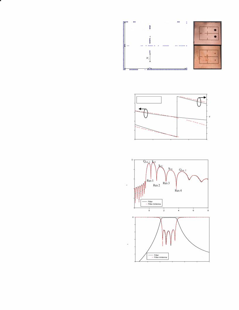
Simulator (HFSS). The filter responses are presented in Fig. 4b. The simulated center frequency, bandwidth, and insertion loss are, 9.85 GHz, 6.5%, and 0.53 dB, respectively. Return losses better than 17 dB are achieved within the entire passband.

B.Slot Antenna Synthesis

In order to replace one port of filter with an antenna mimicking the same effect on the filter as a port, an antenna with a bandwidth wider than the filter bandwidth needs to be chosen. Under this condition, the antenna acts like a load seen from the filter. The coupling to the antenna has to be the same as that to the port. In addition, the frequency loading effect from the antenna needs to be taken into account. If all these factors are properly considered, the designed filter/antenna will have the same filtering function as the original filter.

A frequency-domain analysis is performed first to design the slot antenna. A waveguide port with a width Wand a height of 3.17 mm is set at the reference plane denoted in Fig. 2a. In this simulation setup, the vias at the reference plane are removed. The design procedure is described as follows. (1) Adjust La and Pa to achieve the same Sll magnitude as the coax feeding case. The L,/Pa values can be found using parametric sweeps of the two variables. It is noted here that there is no unique solution, i.e. there may be many different combinations of the two parameters to achieve the same Sll magnitude. Since the slot antenna has a much wider bandwidth than the filter, a slightly different La can still cover the filter bandwidth. (2) Adjust L.J to achieve the same Sll phase as the coax feeding case. As shown in Fig. 3, it is apparent that both the magnitude and phase of Sll match closely for the two different terminations, particularly around the design center frequency.

The frequency-domain synthesis leads to filter/antenna structure dimensions which give a reasonably good Sll response. Fine tuning is still necessary to close the synthesis loop. Since full-wave simulations of this 3-D filter/antenna structure are computationally expensive, a time-domain filter tuning technique [6] is used here. This time-domain technique is able to fine-tune the filter responses with just a few parametric sweeps. Using an inverse Chirp-Z transform, the filter Sll response is plotted in the time domain as shown in Fig. 4a. It is observed that the filter response from different sections of the filter is isolated in the time-domain. The peaks in the time-domain response correspond to the external

coupling at Port 1, the internal coupling between resonators 1 and 2 (k12), k23, k3.J, and the external coupling at Port 2,

respectively, from left to right. The dips correspond to the resonators 1 through 4, respectively. A rise/sink of the level of

the peaks means too small/too large coupling. While the rise of the dips from their minimum values means off-tuned resonances. Following the guideline in [6], the filter/antenna Sll time-domain response can be tuned to match that of the equivalent filter. It is found that: L2 is increased by 100 /lm to

L3 to match the dip of Resonator 3; WI is decreased by 200 /lm to W3 to match k3.J; L.J is fine-tuned to 9.6 mm to the match the dip of Resonator 4; and LjPa is fine-tuned to 12.2/2.3 mm to

match Qext, 2. The Sll of the filter/antenna system in both time­ and frequency-domains are illustrated in Fig. 4. Excellent agreement between the filter and filter/antenna is apparent.

III. RESULTS AND DISCUSSION

A prototype filter and filter/antenna are fabricated and measured to verify the synthesis described in Section II. The photos of the fabricated devices are shown in Fig. 1 and 2. SMA connectors are mounted at the feeding via and soldered at the flange on one side of the PCB and the inner conductor on the other side to form a solid connection.

The measured four-pole filter responses are plotted against the simulation results in Fig. 5a. There is a slight (1.1%) frequency shift due to the fabrication tolerances. The measured bandwidth of 6.3% is very close to the simulated bandwidth of 6.5%. Impedance matching is better than 13 dB across the entire passband. The measured insertion loss of 0.5 dB is slightly lower than the simulated 0.53 dB. This favorable difference is very likely due to the actual lower loss tangent of the substrate material. This low insertion loss of the filter corresponds to a resonator Q factor around 1,000 in Xband.

The measured filter/antenna responses are plotted against the simulation results in Fig. 5b. Again there is a 1.1% frequency shift. It is noted that the consistency between fabricated devices is quite good. The center frequency of the filter and filter/antenna coincides quite closely. The measured filter/antenna bandwidth of 6.0% is slightly less than the simulated 6.5%. The matching is better than 15 dB within the passband. The measured radiation patterns agree very well with the simulation results (Fig. 6) in both E- and H-planes at the center frequency. Similar radiation patterns are observed across the entire passband. It is noted that the pattern in E­ plane has a slight dip at the boresight. This may be caused by the close proximity of the ends of the slot antenna to the sidewalls of the resonator. This adverse effect can be removed by improved designs. The measured maximum gain is 6.1 dB. The efficiency of the integrated filter/antenna system is calculated using GainiDirectivity and found to be 89%, which is equivalent to a 0.51 dB loss. The directivity is simulated using HFSS. This efficiency is very close to the measured