книги2 / 46

MODELLING OF AIR PRESSURE DYNAMICS FOR CLEAN ROOM FACILITIES

S. Horngacher, M. Kozek

Vienna University of Technology, Vienna, Austria

Corresponding Author: M. Kozek, Vienna University of Technology, Inst. f. Mechanics and Mechatronics Wiedner Hauptstraße 8 - 10, 325A5, 1040 Wien, Austria; martin.kozek@tuwien.ac.at

Abstract. In the pharmaceutical industry strict specifications concerning overpressure and actively overpressure controlling should guarantee that only preconditioned air enters clean room facilities. A modular and easily to parameterize model is created in Simulink to describe the system dynamics and to avoid pressure surges, which occur when doors between different control zones are closed. In addition to state of the art mathematical modelling, which is based on non-stationary mass balances and basic thermodynamic equations, the strongly non-linear behaviour of some components is identified from experimental data of a laboratory test set-up and of the real plant. Experimental validation shows excellent results. The phenomenon “pressure surge” turns out to be the consequence of integral controller action and measurement bias, which was proven by both the model prediction and measurements.

1 Introduction

In the pharmaceutical industry clean room pressure is important in terms of product quality, because overpressure guarantees that only preconditioned air enters the facilities. Strict specifications prescribe overpressure and differential pressure between different clean room classes. Therefore, the pressure has to be actively controlled. When doors between different control zones are closed, pressure surges occur and the pressure may exceed specified limits.

There already exist multi-zone air flow models, which model the air flow and contaminant distribution in buildings [2]. They are quite extensive and for simulation require solving an overall mass balance for the whole building. Most existing models focus on air conditioning and ventilation technologies, where air flows through doors are not implemented and energetic considerations are most important [1], [3-5].

The motivation for the work presented here is to create a modular and easy to parameterize model in Simulink, which covers the dynamics of the system and the cause of the phenomenon “pressure surge”. Moreover, the model should be a basis for testing different control concepts in terms of robust pressure control.

The mathematical modelling follows state of the art procedures using non-stationary mass balances and basic thermodynamic equations. Ventilation facilities and pipe networks are idealized and air flows through doors are implemented. In order to apply the model to a realistic room topology detailed experimental identification of actuation devices was performed in laboratory, pointing out the strongly nonlinear behaviour of the actuator. Additionally, measurements at the clean room facilities were used for parameter optimization and model validation.

The paper is structured as follows: The next section is dedicated to the derivation of the governing equations for the component modelling. Section 3 deals with the component modelling itself and its validation. Results are presented in section 4, whereas section 5 concludes the contents of the paper.

2 Theoretical component modelling

2.1Non-stationary mass balance

The modular simulation model enables a flexible adaptation to a given topological map of rooms. It is based on a non-stationary mass balance for each room i and the ideal gas law, where temperature T and density are considered to be constant and the room volume is a dominant model parameter.

In (1) mi denotes the total air mass of room i, miz denotes the supply air mass flow rate of room i, mia denotes the exhaust air mass flow rate of room i, mij denotes the mass flow rate from room i to adjoining room j, milk de-

notes the leakage flow rate k of room i (more than one leakage flow may be present). The ideal gas law is given by

146

Proceedings MATHMOD 09 Vienna - Full Papers CD Volume

where pi denotes the pressure of room i, Vi denotes the volume of room i, R denotes the specific ideal gas constant of air, T denotes the absolute temperature.

This leads to a linear 1st-order differential equation for the pressure of each room:

haust air volume flow rate of room i, Qij denotes the volume flow rate from room i to room j, Qilk denotes the

leakage volume flow rate k of room i. Note that volume and mass flow rates of air can be easily converted into each other due to the assumption of constant air density ρ .

2.2Flow resistance

Volume flow rates through doors and for leakages are modelled with equations (4) to (7).

p j denotes the pressure of room i, and Rij ,δ k denote adaptation parameters. The power function in (4) allows

for a flexible flow resistance model which can be easily fitted to measured data. Leakage flow rates are modelled similar

where pu denotes 1e5 Pa (ambient pressure), and Rilk ,γ ilk denote adaptation parameters.

The actuator is a continuously variable ventilation flap (clack valve) with electric drive positioned at the exhaust air duct. The strongly nonlinear behaviour of the actuator is modelled by a 3-point controller with hysteresis (dead and neutral zone) (see also Fig. 3a.), as well as a nonlinear static characteristic (see also Fig. 3b.):

In (8) pi,clack denotes the pressure difference of room i at the actuator, α i denotes the actuating variable of room i (angle of clack valve i), Ri (α i ) denotes a regression function which was fit to experimental data depending on the actuating variable of room i, and β i denotes an adaptation parameter.

The parameters of those nonlinear elements and the limited rate of the actuator were identified at a laboratory test set-up.

The pressure sensor is a ring balance, and it is modelled as a PT1 element (9) with gain one, whose time constant results from experiments at the real plant. Measurement bias is added to the room pressure signal (10).

Gi,rb denotes the ring balance transfer function of room i, Ti denotes the ring balance time constant of room i, pirb denotes the delayed measurement of the ring balance of room i, pim denotes the measured pressure of room i, bi denotes the measurement bias of room i,

Validation facilities and duct systems are idealized. Supply air and exhaust air are modelled by an ideal flow and pressure source, respectively. There is one plenum for the supply air and one for the exhaust air. The same equa-

147

tions are used as for the rooms. The volume flow rate of all the supply air into the rooms and of the exhaust air out of the rooms at 105 Pa is considered and kept constant by a flow controller (see Fig. 1).

3Component modelling

One ventilation system (Fig. 1) represents the basic structure to demonstrate the phenomenon “pressure surge”. It consists out of the following modules: One plenum for the supply air, one plenum for the exhaust air, two rooms at 1,0002·105 Pa connected with one door and independently controlled by PI controllers, which manipulate the volume flow rate of the exhaust air, and one room module which represents all the other rooms of the ventilation system at 105 Pa. The volume flow rates of supply and exhaust air are assumed to be kept constant by a flow rate controllers (Fig. 1).

PLENUM 2 FOR THE EXHAUST AIR

IDEAL EFFORT

Figure 1. Overall model scheme of one ventilation system

To validate the theoretical model, this structure of rooms was used for experiments at the real plant, where data logging of the additionally monitoring sensors and high-bandwidth sensors were implemented in addition to the control sensors. All pressure data were logged every 2s and the data of the actuating variables were logged every 60s.

3.1Module “room”

All mathematical models for room modules are based on equation (3). The density = 1,2 kg/m3, the specific ideal gas constant of air R=287J/kgK, and the temperature T=296,15K are considered to be constant. Using these assumptions the following differential equations result:

148

Proceedings MATHMOD 09 Vienna - Full Papers CD Volume

Qpl1_ 1z ,Qpl1_ 2z ,Qpl1_ 3z denote the supply air ideal volume flow rates, which are taken equal to measured values of the real plant.

k

V1, V2 and V3 are given by a topological map. Vpl1 and Vpl2 were identified from experimental data.

The operating point for rooms 1 and 2 is 1,0002·105 Pa, that is 20 Pa overpressure. The operating point for the other rooms of the ventilation system is 105 Pa, and it is constant in the simulation model, because of flow controllers for supply and exhaust air, which keep the supply and exhaust volume flow rate constant. Pressures for the plenum of the supply air and the one of the exhaust air result from the simulation.

Table 1. Model parameters for the module “room”

3.2Module “actuator”

The basic model structure of the actuator was taken from the manufacturer’s manual. The parameters of the hysteresis which are a dead and neutral zone, as well as the limited rate of the actuator result from measurement data of a laboratory test set-up, which represents a characteristic configuration of an air exhaust duct (Fig. 2). During the validation process the parameters of the hysteresis (see Fig. 3a.) had to be adapted for the actuators of the real plant in order to get satisfying simulation results.

149

Figure 2. Laboratory test set-up

In room 1 the pipe diameter of the exhaust duct d1 =160mm corresponded to the one of the test set-up. Values of the following two functions were measured

f denotes the frequency of the fan of the test set-up.

By eliminating the frequency, the nonlinear static characteristic of room 1 was obtained (Fig. 3b.)

and the parameters of R1( 1) and 1 were identified from a logarithmic regression:

a1 , a2 , a3 , a4 denote the respective regression parameters.

Because the exhaust duct of room 2 had a different pipe diameter d2 =200mm, its characteristic static function had to be generated out of measured data of the real plant.

Again, b1 ,b2 ,b3 ,b4 denote regression parameters. The numerical values of these models are listed in Table 2.

150

Proceedings MATHMOD 09 Vienna - Full Papers CD Volume

Table 2. Model parameters for the module “actuator”

3.3Module “door”, module “leakage”

Volume flow rates through doors and for leakages are modelled with equations (4) to (7). During the first experiment at the real plant the controllers of room 1 and 2 were inactive (open loop). All the doors (door between room 1 and 2, two air lock doors of room 2) and a pass-through of room 1 were sealed. The describing equations for leakages are given by:

Q1l1 denotes the leakage volume flow rate of room 1, when the door between room 1 and 2 and the pass-through of room 1 are sealed.

Q1l 2 denotes the leakage volume flow rate of a pass-through of room 1.

151

Q2l1 denotes the overall leakage volume flow rate of room 2, where the door between room 1 and 2 is sealed, but not the two air lock doors.

When the sealings were successively removed, the parameters R12, R1l1, R1l2, R2l1, 1, 1l1, 1l2 and 2l1 in equations (17) to (22) were identified from step responses.

Table 4. Model parameters for the module “sensor”

3.5Module “PI controller”

The PI controllers at the real plant have a given cycle time of 10s and a dead zone of ±0,6Pa, which was also implemented in the simulation model. The dead zone suppresses actuator action caused by the propagation of measurement noise in the control loop. Numerical values of the controller parameters are withheld due to confidentiality. However, from the comparatively large cycle time of the control loop it is obvious that fast dynamics like the pressure surge cannot be compensated by closed loop control action.

152

Proceedings MATHMOD 09 Vienna - Full Papers CD Volume

4 Results

The experiment at the real plant presented here was performed to analyze the phenomenon “pressure surge”. The room topology at the clean room facilities corresponds to the scheme given in Fig. 1 (two independently controlled adjacent rooms with a connecting door). At first, stationary undisturbed operation with door closed was ensured (time span form t=4500s to t=4920s). At t=4920s the connecting door was opened and held open until t=6500s. At that time instant the door was closed again and the measurement was continued until stationary operation was reached again.

It is important to notice that the measured room pressures of the ring balances are biased, and therefore, during stationary operation a difference between the actual individual room pressures exists. As a consequence, only the measured values of the room pressures are close to the set point of 20 Pa overpressure at the beginning of the experiment.

The connecting door between the two rooms was opened at 4920s. From that time instant on, there are two actuating variables for just one controlled variable (the open door effectively creates one single room with the joint volume of both rooms). The system becomes undefined and unstable due to the combined integral controller action and measurement bias. Although the overpressure could be held around 20 Pa, the actuating variables drifted apart (Fig. 4b) and the simulation shows that the volume flow rate through the door increases over time (Fig. 5a). One of the actuating variables reached the saturation of 80% at approximately t=5470s, the other actuating variable remained constant from t=5750s (Fig. 4b). Since the connecting door was wide open at this stage of the experiment the actual room pressure must have been almost identical. Instead, the measured room pressures are 19,8 Pa and 21.6 Pa, respectively (Fig. 4a). This difference is caused by the combined pressure bias of both rooms.

Figure 4. Phenomenon “pressure surge” – door opening at 4290s, door closing at 6500s

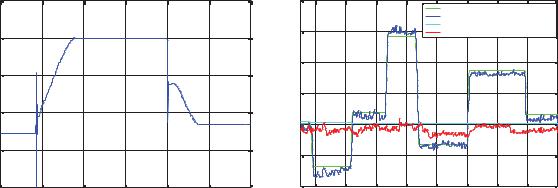
At t=6500s the door was closed and the actuators were both in an offset position compared to the stationary case. A strong air flow through the connecting door existed at that stage (Fig. 5a). Therefore, a pressure surge was the consequence (Fig. 4a). Both measured and simulated pressure signals are output values of the ring balances which are low-pass elements (see section 3.4). The actual pressure surge reaches considerably higher actual pressure values, however, it is of very short duration and therefore not recorded and considered.

Note that the measured actuating variable of room 2 had an offset due to a faulty ring balance (Fig. 4b). The remaining difference in room pressures at the end of the experiment (Fig. 4a) is caused by the dead zone of the actuators.

The room module itself turns out to be a quasi static model. The slope of step responses of the real plant corresponds to the limited rate of the actuator, which indicates that the room pressure acts synchronously to the position of the actuator (Fig. 5b). The fast dynamics of the systems were proven by high-bandwidth pressure sensors in a separate experiment (Fig. 5b), where an additional reference measurement with poor stationary accuracy but low cost effort was implemented on the plant. Because of the “slow” element in the system, which obviously is the ring balance with its PT1 behaviour (see section 3.4), the speed at which the door is closed doesn’t affect the measured results.

Comparison of measured to simulated data shows that the model covers both the system dynamics and the phenomenon “pressure surge” (Fig. 4 and 5b).

153

Figure 5. a. Phenomenon “pressure surge” – door opening at 4290s, door closing at 6500s, b. Step responses caused by the actuating variable of room 1

5 Conclusion

Only preconditioned air is allowed to enter clean room facilities in the pharmaceutical industry. Therefore, actively controlled overpressure is maintained and should not exceed specified limits, which might occur in case of pressure surges when closing doors between different clean room classes.

State of the art mathematical modelling and measurement data of a laboratory test set-up and the real plant lead to a modular simulation model of low order. It covers the system dynamics and the phenomenon “pressure surge”. The model can be easily parameterized and applied to a realistic room topology. Therefore, manuals or measurement data are sufficient to provide the parameters and the nonlinear static characteristic of the actuator.

On the basis of this model different controller concepts will be implemented in Simulink and evaluated in terms of robustness in order to avoid pressure surges.

6References

[1]Hisashi Yamasaki, Toshiyuki Watanebe, Hitoshi Yamazaki. VAV air conditioning system simulation controlling room air temperature, humidity and pressure. J Archit Plann Environ Eng, 2001, 548: 37 - 43

[2]http://gsb.download.bva.bund.de/BBK/Zivilschutz_Bd_39.pdf

[3]Kazuhiro Yamashita, Tathuo Gotoh, Hitoshi Yamazaki. Study on air conditioning simulations for rooms and duct systems. J Archit Plann Environ Eng, 1998, 507: 21 - 26

[4]Tanaka D., Koike T., Tanaka N., Miyake T., Tateno S., Matsuyama H. A study on design review of the control performance of the air conditioning to prevent room pressure change troubles.[Conference Paper] 2006 SICE-ICASE International Joint Conference (IEEE Cat. No. 06TH8879). IEEE. pp. 6. Piscataway, NJ, USA.

[5]Wu Chen, Shiming Deng. Development of a dynamic model for DX VAV air conditioning systems. Energy Conversion and Management, 2006, 47:2900 - 2024

154