Добавил:

a_lex_71 Опубликованный материал нарушает ваши авторские права? Сообщите нам.

Вуз:

Национальный исследовательский университет «МИЭТ»

Предмет:

Системное проектирование в телекоммуникациях

Файл:

4 семестр ИКТ 6 вариант / ЛР6 СПВТ

.docx

Скачиваний:

Добавлен:

21.02.2024

Размер:

963.35 Кб

Скачать

☆

Лабораторная работа №6

Задание 1

clc; clear; close all;

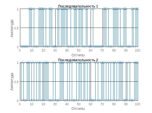
N=100;

goldseq1 = comm.GoldSequence('FirstPolynomial','x^6+x+1','SecondPolynomial','x^6+x^5+x^2+x+1','FirstInitialConditions',[0 0 0 0 0 1],...

'SecondInitialConditions',[0 0 0 0 0 1],'Index',0,'SamplesPerFrame',N);

goldseq2 = comm.GoldSequence('FirstPolynomial','x^6+x+1','SecondPolynomial','x^6+x^5+x^2+x+1','FirstInitialConditions',[0 0 0 0 0 1],'SecondInitialConditions',[0 0 0 0 0 1],'Index',10,'SamplesPerFrame',N);

x1 = step(goldseq1); x2 = step(goldseq2);

figure;

subplot(2,1,1);

stem(x1);

grid on;

xlabel('Отсчеты');

ylabel('Амплитуда ')

title('Последовательность 1');

subplot(2,1,2);

stem(x2);

grid on;

xlabel('Отсчеты');

ylabel('Амплитуда')

title('Последовательность 2');

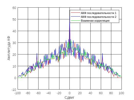
[r1,lags1]=xcorr(x1);

[r2,lags2]=xcorr(x2);

[r3,lags3]=xcorr(x1,x2);

figure;

plot(lags1,r1,'r')

hold on;

grid on

plot(lags2,r2,'b');

plot(lags3,r3,'g')

xlabel('Сдвиг');

ylabel('Амплитуда КФ')

legend('АКФ последовательности 1','АКФ последовательности 2','Взаимная корреляция')

clc; clear; close all;

Fs = 5e3;

T = 1/Fs;

N = 10000;

t = (0:N-1)*T;

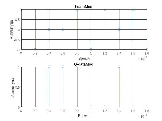
M=4;

data=randi([0 M-1],N,1);

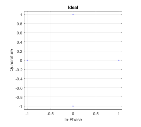
dataMod = pskmod(data,M);

scatterplot(dataMod)

grid on

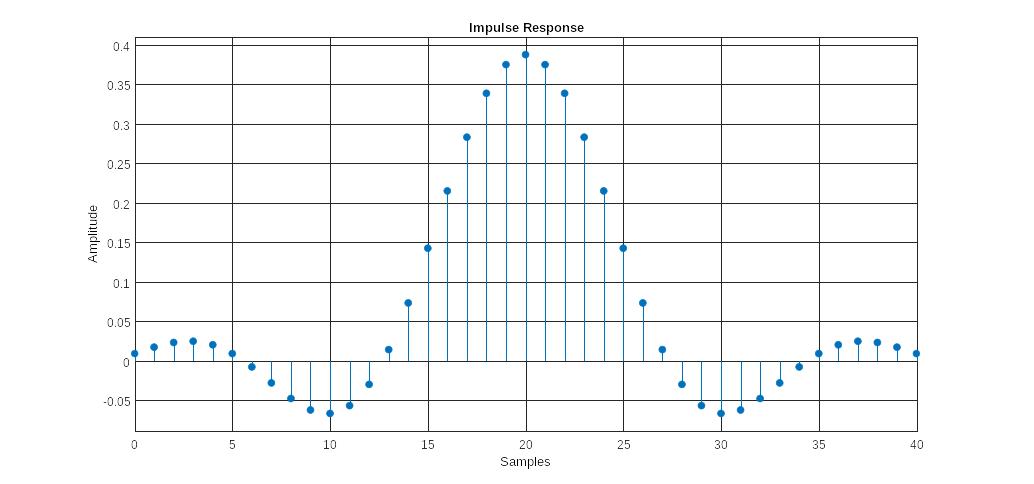
Nsamp=8;

rolloff = 0.35;

span = 5;

b = rcosdesign(rolloff, span, Nsamp);

dataModRC = upfirdn(dataMod, b, Nsamp);

fvtool(b,'Impulse')

Fs = 5e3;

T = 1/Fs;

N = 10000;

t = (0:N-1)*T;

M=4;

data=randi([0 M-1],N,1);

dataMod = pskmod(data,M);

n=10;

figure; subplot(2,1,1);

stem(t(1:n),real(dataMod(1:n)));

title('I-dataMod');xlabel('Время');

ylabel('Амплитуда'); grid on;

subplot(2,1,2);

stem(t(1:n),imag(dataMod(1:n)));

title('Q-dataMod');xlabel(' Время ');

ylabel(' Амплитуда '); grid on;

figure; subplot(2,1,1)

stem(T/Nsamp*(1:n*Nsamp),real(dataMod(1:n*Nsamp)));

title('I-dataModRect'); xlabel(' Время ');

ylabel('Амплитуда'); grid on;

subplot(2,1,2);

stem(T/Nsamp*(1:n*Nsamp),imag(dataMod(1:n*Nsamp)));

title('Q-dataModRect'); xlabel(' Время ');

ylabel('Амплитуда'); grid on;

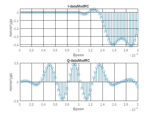
figure; subplot(2,1,1)

stem(T/Nsamp*(1:n*Nsamp),real(dataModRC(1:n*Nsamp)));

title('I-dataModRC');xlabel(' Время ');

ylabel('Амплитуда'); grid on;

subplot(2,1,2);

stem(T/Nsamp*(1:n*Nsamp),imag(dataModRC(1:n*Nsamp)));

title('Q-dataModRC');xlabel(' Время ');

ylabel('Амплитуда'); grid on;

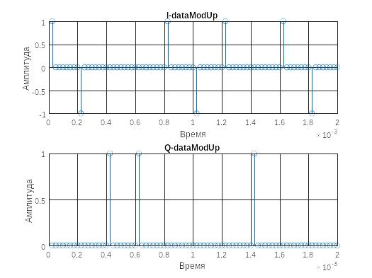
dataModUp=upsample(dataMod,Nsamp);

figure; subplot(2,1,1); stem(T/Nsamp*(1:n*Nsamp),real(dataModUp(1:n*Nsamp)));

title('I-dataModUp');xlabel('Время');

ylabel(' Амплитуда '); grid on;

subplot(2,1,2); stem(T/Nsamp*(1:n*Nsamp),imag(dataModUp(1:n*Nsamp)));

title('Q-dataModUp');xlabel(' Время ');

ylabel(' Амплитуда '); grid on;

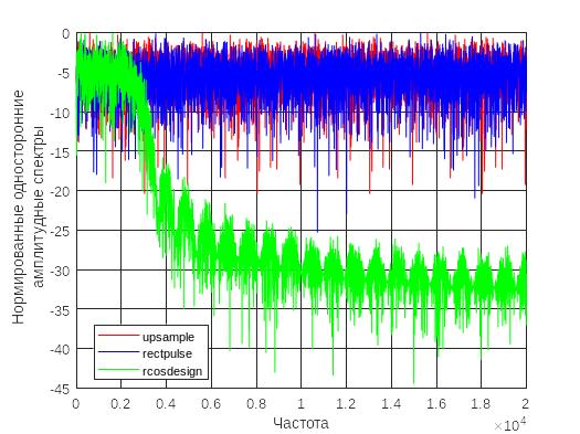
Nfft=8096;

Y(:,1) = fft(dataModUp,Nfft);

Y(:,2) = fft(dataMod,Nfft);

Y(:,3) = fft(dataModRC,Nfft);

P2 = abs(Y/Nfft);

P1 = P2(1:Nfft/2+1,:);

P1(2:end-1,:) = 2*P1(2:end-1,:)

Fs2=Fs*Nsamp;

f2 = Fs2*(0:(Nfft/2))/Nfft;

figure;

plot(f2,10*log10(P1(:,1)./max(P1(:,1))),'r',f2,10*log10(P1(:,2)./max(P1(:,2))),'b',f2,10*log10(P1(:,3)./max(P1(:,3))),'g')

grid on

xlabel('Частота');

ylabel({'Нормированные односторонние','амплитудные спектры'});

legend('upsample','rectpulse','rcosdesign','Location','best')

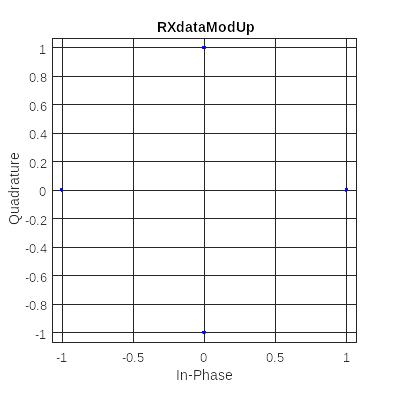
RXdataModUp=downsample(dataModUp,Nsamp);

RXdataModRect = intdump(dataMod,Nsamp);

RXdataModRC = upfirdn(dataModRC, b,1, Nsamp);

RXdataModRC =RXdataModRC (span+1:end-span);

scatterplot(RXdataModUp); grid on;

title('RXdataModUp')

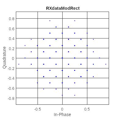
scatterplot(RXdataModRect); grid on;

title('RXdataModRect')

scatterplot(RXdataModRC); grid on;

title('RXdataModRC')

clc; clear; close all;

N = 1000000; p = 0.5;

y1 = wgn(N,1,p,'linear','complex');

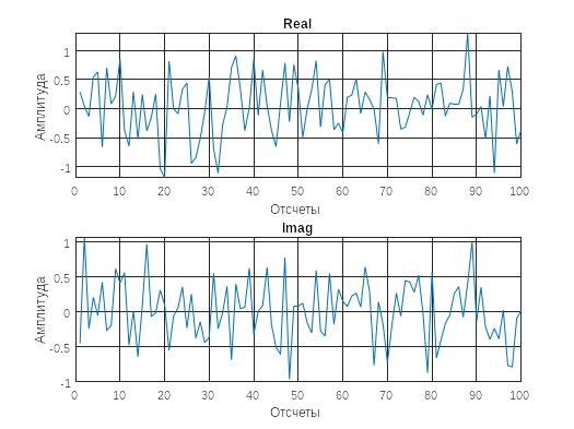
figure; subplot(2,1,1)

plot(real(y1)); grid on;

xlabel('Отсчеты'); title('Real')

ylabel(' Амплитуда ')

subplot(2,1,2)

plot(imag(y1)); grid on;

xlabel(' Отсчеты '); title('Imag')

ylabel('Амплитуда');

subplot(2,1,1)

xlim([0 100])

subplot(2,1,2)

xlim([0 100])

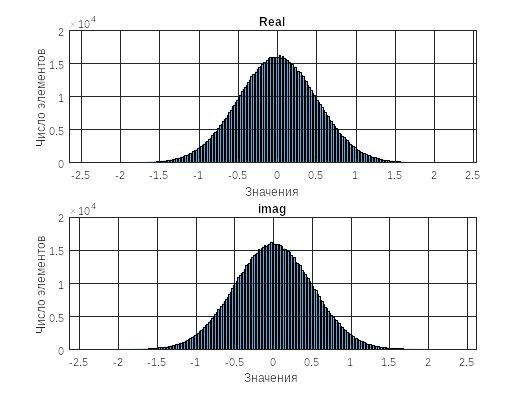
figure; subplot(2,1,1)

histogram(real(y1));grid on

xlabel('Значения'); title('Real')

ylabel('Число элементов')

subplot(2,1,2)

histogram(imag(y1)); grid on

xlabel(' Значения '); title('imag')

ylabel(' Число элементов ')

Fs = 20e3; Nfft=4096;

Y = fftshift(fft(y1,Nfft)); P2 = abs(Y./Nfft);

f1 = linspace(-Fs/2,Fs/2,Nfft);

figure; plot(f1,10*log10(P2))

grid on; xlabel('Частота')

ylabel('Амплитуда')

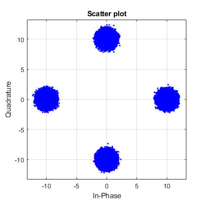
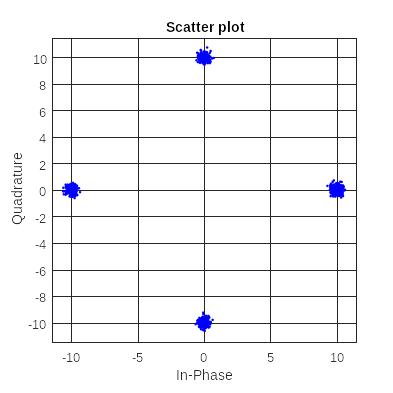
M=4;

data=randi([0 M-1],N,1);

dataMod = 10*pskmod(data,M);

N = 1000000; p = 0.5;

y1 = wgn(N,1,p,'linear','complex');

scatterplot(y1+dataMod)

grid on

clc; clear; close all;

N = 1000000; p = 0.5;

y1 = wgn(N,1,p,'linear','complex');

Fs = 20e3;

Nfft=4096;

Y = fftshift(fft(y1,Nfft));

P2 = abs(Y./Nfft);

f1 = linspace(-Fs/2,Fs/2,Nfft);

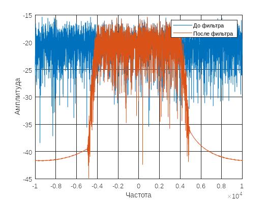
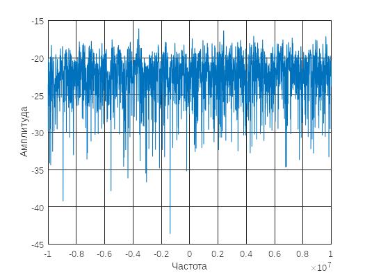
figure;

plot(f1,10*log10(P2))

grid on;

xlabel('Частота')

ylabel('Амплитуда');

hold on

y2=filter2(y1);

Y2 = fftshift(fft(y2,Nfft));

P22 = abs(Y2./Nfft);

plot(f1,10*log10(P22))

legend('До фильтра','После фильтра')

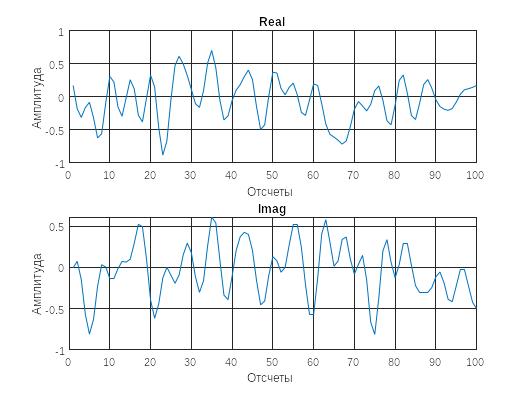
figure; subplot(2,1,1)

plot(real(y2));

grid on;

xlabel(' Отсчеты ');

title('Real')

ylabel(' Амплитуда ');

xlim([0 100])

subplot(2,1,2)

plot(imag(y2));

grid on;

xlabel(' Отсчеты ');

title('Imag')

ylabel(' Амплитуда ');

xlim([0 100])

T=1/Fs;

t = (0:N-1)*T;

M=4;

SNR=30;

N=1000;

data=randi([0 M-1],N,1);

dataMod = 10*pskmod(data,M);

dataModAwgn = awgn(dataMod,SNR,'measured');

scatterplot(dataModAwgn);

grid on;

figure;

stem(t(1:N)/N,data(1:N,1))

hold on

stem(t(1:N),data(1:N,1),'LineWidth',2)

xlabel('Время');ylabel('Амплитуда')

y = pskmod(data,M);

Fs2=Fs*N;

Y1 = fftshift(fft(y,Nfft));

P1 = abs(Y1/Nfft);

f1 = linspace(-Fs2/2,Fs2/2,Nfft);

figure; plot(f1,10*log10(P1))

hold on; xlabel('Частота');

ylabel('Амплитуда');

grid on

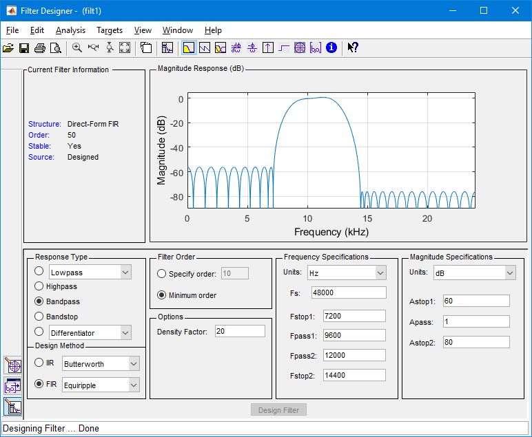
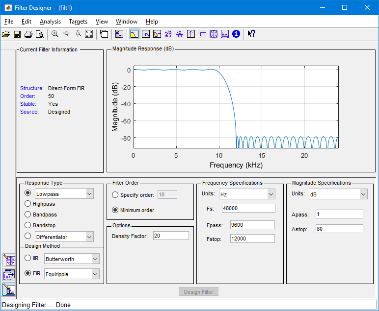
Создаем м-файл с помощью file-generete matlab code

function y = bandpass_filter(x)

%BANDPASS_FILTER Filters input x and returns output y.

% MATLAB Code

% Generated by MATLAB(R) 9.7 and DSP System Toolbox 9.9.

% Generated on: 11-Jun-2021 00:29:38

%#codegen

% To generate C/C++ code from this function use the codegen command. Type

% 'help codegen' for more information.

persistent Hd;

if isempty(Hd)

% The following code was used to design the filter coefficients:

% % Equiripple Bandpass filter designed using the FIRPM function.

% % All frequency values are in Hz.

% Fs = 48000; % Sampling Frequency

% Fstop1 = 7200; % First Stopband Frequency

% Fpass1 = 9600; % First Passband Frequency

% Fpass2 = 12000; % Second Passband Frequency

% Fstop2 = 14400; % Second Stopband Frequency

% Dstop1 = 0.001; % First Stopband Attenuation

% Dpass = 0.057501127785; % Passband Ripple

% Dstop2 = 0.0001; % Second Stopband Attenuation

% dens = 20; % Density Factor

% % Calculate the order from the parameters using FIRPMORD.

% [N, Fo, Ao, W] = firpmord([Fstop1 Fpass1 Fpass2 Fstop2]/(Fs/2), [0 1 ...

% 0], [Dstop1 Dpass Dstop2]);

% % Calculate the coefficients using the FIRPM function.

% b = firpm(N, Fo, Ao, W, {dens});

Hd = dsp.FIRFilter( ...

'Numerator', [0.000405311015767794 -0.000340162424744898 ...

-0.00275017457650894 -0.00174274245080288 0.00514491904143094 ...

0.00647577832444998 -0.00568854990170438 -0.0126842654631062 ...

0.00248179604874337 0.0160107744241188 0.00223850273897986 ...

-0.0125757061527468 -0.0014127959970525 0.00406157889441876 ...

-0.0126642406219731 -1.85837801898815e-05 0.0408268777064353 ...

0.0133647214892565 -0.0722859420326916 -0.0505173101841354 ...

0.0883091271404975 0.103364573239606 -0.0737806038715708 ...

-0.150637807286995 0.0288308946921712 0.169635266121261 ...

0.0288308946921712 -0.150637807286995 -0.0737806038715708 ...

0.103364573239606 0.0883091271404975 -0.0505173101841354 ...

-0.0722859420326916 0.0133647214892565 0.0408268777064353 ...

-1.85837801898815e-05 -0.0126642406219731 0.00406157889441876 ...

-0.0014127959970525 -0.0125757061527468 0.00223850273897986 ...

0.0160107744241188 0.00248179604874337 -0.0126842654631062 ...

-0.00568854990170438 0.00647577832444998 0.00514491904143094 ...

-0.00174274245080288 -0.00275017457650894 -0.000340162424744898 ...

0.000405311015767794]);

end

y = step(Hd,double(x));

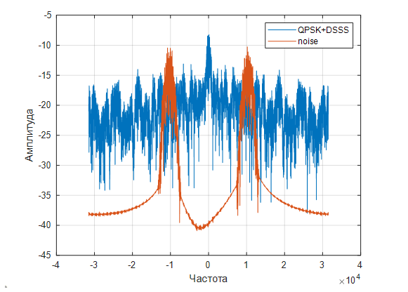
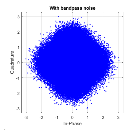
Ibandpass_noise=bandpass_filter(wgn(length(y),1,5));

Rbandpass_noise=bandpass_filter(wgn(length(y),1,5));

bandpass_noise=1i*Ibandpass_noise+Rbandpass_noise;

Y2 = fftshift(fft(bandpass_noise,Nfft));

P2 = abs(Y2/Nfft);

plot(f1,10*log10(P2))

legend('QPSK+DSSS','noise')

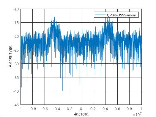
Y2 = fftshift(fft(y+bandpass_noise,Nfft));

P2 = abs(Y2/Nfft);

figure;

plot(f1,10*log10(P2))

hold on; xlabel('Частота');

ylabel('Амплитуда'); grid on

legend('QPSK+DSSS+noise')

Rxy = pskdemod(y+bandpass_noise,M);

Rxy1=de2bi(Rxy);

Rxy2=xor(Rxy1(:),repmat(x1,N,2));

Rxdata = round(intdump(double(Rxy2),Ng));

[number, ratio]=biterr(data,Rxdata)

Rxy = pskdemod(y+bandpass_noise,M);

Rxy1=de2bi(Rxy);

Rxy2=xor(Rxy1(:),repmat(x1,N,1));

Rxdata = round(intdump(double(Rxy2),Ng));

[number, ratio]=biterr(data,Rxdata)

number = 0

ratio = 0

number = 0

ratio = 0

Соседние файлы в папке 4 семестр ИКТ 6 вариант

#
21.02.20241.64 Mб0кр2 спвт_2.jpg
#
21.02.202471.95 Кб0лаба 2 спвт.docx
#
21.02.2024236.45 Кб0ЛР3 СПВТ.docx
#
21.02.2024243.62 Кб0ЛР4 СПВТ.docx
#
21.02.2024870.67 Кб0ЛР5 СПВТ.docx
#
21.02.2024963.35 Кб0ЛР6 СПВТ.docx
#
21.02.2024278.91 Кб0ЛР7 СПВТ.docx
#
21.02.2024265.46 Кб0ЛР8 СПВТ.docx