932

compared with the soil erosion obtained from the G2loss model.

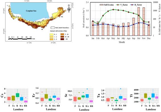
Results and Discussion. Land use contribution in soil erosion. The annual maps of G2loss inputs including R (MJ mm ha-1 h-1), V, S, T, and L factors are shown in Fig. 2. The lower and higher annual R valuesin the study area are equal to 34.61 and 564.20 MJ mm ha-1 h-1, respectively. The average R without the snow correction coefficient is equal to 307.31, and with the snow correction coefficient is equal to 245.75. Therefore, due to the effect of the snow cover on the ground during some months in the study area,

rainfall erosivity was reduced. The V factor value ranged from 1 to 4438.82 and the average annual V factor of the study area was 523.19. The positive effect of vegetation cover in the Hyrcanian forests in the Iranian part of the Caspian Sea Basin prevents soil loss in this region. While in the south and southeastern parts of thebasins,subthe

vegetation retention factor is close to one and indicates poor vegetation cover, and consequently, the soil protection caused by vegetation cover is much less than in the forest areas [18, 24].

Fig. 2. The Annual maps of G2loss model inputs in the study area (a: Rainfall erosivity; b: Vegetation retention; c: Soil erodibility; d: Terrain influence; e: Landscape effect)

The S factor value in the study arearanged from zero (no soil areas) to 0.045, with an average of 0.036 (t h MJ-1 mm-1). Most of the dominant soils in the south of the study

area have less than 3% organic carbon. These soils are located in the highlands where rangeland is the main land use and the soils have a relatively weak structure and high erodibility and are sensitive to erosion [8]. The T factor value varied from 0.01 to 133.5.

The lowest value of T factor is related to flat areas [1], while the highest values of T factor

are related to steep and high areas (Alborz Mountains). The undeniable effect of topographical factors on soil erosion has been mentioned in previous studies [23]. The value

401

of average annual L factor in the study area was 1.71. As a result of poverty or lack of vegetation, as well as dry soil and heavy rainfall, the numerical value of the L factor decreases, this indicates more soil erosion [11]. The annual soil erosion (t ha-1) map of the

study area is shown in Fig. 3. The average annual soil erosion estimated for the study area was 13.46 t ha−1. The highest erosion rate in the study area is located in the upstream parts, where the highest slope gradients have low vegetation retention values in the southern parts [8]. The results of this study are in agreement with previous studies which indicated the rate of soil erosion in the north of Iran between 0 and 20 -t1 hayr-1 [2, 18]. The relationship between average monthly soil erosion, R and V factors are shown in Fig. 4.

Based on the results, from April to August, because of more V and less R, the soil erosion is less, but in other months, especially in October and November, the V and the R is less and more, respectively, and the soil erosion rate is high (Fig. 4).

Land use contributions in sediment yield. The boxplots of the average concentration of the optimal geochemical tracers are shown in Fig. 5.

Fig. 5. Boxplot of the average concentration of the optimal geochemical tracers (mg kg-1) in the Talar Watershed (Note: F “forest”, IA “irrigated agriculture”, R “rangeland”, RA “rainfed agriculture”, and RB “riverbanks”)

The concentration of Ti and Sc tracers were higher in most of the source samples compared to the suspended sediment sample, which is confirmed the findings reported by [17]. The sediment source contributions in the Talar Watershed were obtained using the mixing model. The contribution of rainfed agriculture, irrigated agriculture, rangeland, and forest to suspended sediment yield were 49.9, 35.6, 9.8, and 4.4%, respectively theand GOF index was 57.60%. The specific contribution (per hectare) of different land uses on suspended sediment yield for irrigated agriculture, and rainfed agriculture were higher than the rangeland (Table 1). Accordingly, there is a significant variation in heavy metals concentration (as geochemical tracers) based on flow discharge and human activitiesat different parts of the rivers [5].

402

Integration of G2loss and sediment fingerprinting results/ In most sub-basins of the study area, rangeland, forest, and agriculture have the highest soil erosion rates -1(t), ha respectively. It is very important to note that therangeland mostly located in the steep slope highlands in the south of the sub-basins, with more erodible soils and low vegetation cover compared to the forest which led to increased soil erosion in the rangeland. Finally,Table 2 indicates the annual sediments delivered to the Caspian Sea from the southern sub-basins for the main land uses of forest, rangeland, and agriculture, separately.

Table 1

The specific contribution of land use/land covers in suspended sediment yield of the Talar Watershed

According to Table 2, the contributions of 73.77, 21.74, and 4.49% in annual soil erosion were related to the rangeland, forest,and agriculture, respectively. While the results

of the average contribution of land uses in suspended sediment are opposite and the contributions of 59.97, 28.15, and 19.84% were related to agriculture, forest, and rangeland, respectively. The agricultural lands are usually located in low slope lowlands and also the irrigated agricultural lands are often found in the flat plains near the rivers. Therefore,the contribution of agricultural lands in suspended sediment yield was more than the rangeland

and forest. Also, forest was the second major source of suspended sediment yield in the study area, not only because of more coverage, but also because of forest degradation near roads and rivers due to traffic of agricultural machinery, livestock grazing, andecreational activities, which accelerate soil erosion and sedimentation [16].

Table 2

Annual sediments delivered to the Caspian Sea from the southern sub-basins from the main land uses

Conclusions. Sediment sources or land use/land covers with a larger area do not necessarily have a greater contribution to soil erosion and sediment yield. Forest has occupied the largest area, but the rangeland contributes more to soil erosion, mainly because

403

construction, and recreational activities. The highest contribution in sediment yield in the whole study area is related to agricultural lands with the lowest coverage compared to the forest and rangeland. The agricultural lands are located near the rivers andcontribute more

to sediment yield. In addition, these lands are located in lower elevations with higher rainfall intensity and amount. Therefore, human activities, precipitation, land use, and topography are responsible for the differences in soil erosionand the contribution of the potential sediment sources in the study area. The results of soil erosion estimation and identifying the areas with the highest soil erosion rates using the lossG2model combined

with the results of sediment fingerprinting using geochemical tracers makes appropriate information to be used in large scale management.

References

1.Alamdari, P., Nematollahi, O., Alemrajabi, A.A., 2013. Solar energy potentials in Iran: A Review. Renewable and Sustainable Energy Reviews 21, 778-788.

2.Borrelli, P., Robinson, D.A., Panagos, P., Lugato, E., Yang, J.E., Alewell, C., Ballabio, C., 2020. Land use

and climate change impacts on global soil erosion by water (20152070)- . Proc. Natl. Acad. Sci. U.S.A. 117 (36), 21994-22001.

3.Chavoshi, S., Sulaiman, W.N.A., Saghafian, B., Sulaiman, M.N.B., Abd Mana, L., 2013. Flood prediction in southern strip of Caspian Sea Watershed. Water Resour. Reg. Water Body. 40(6), 593-605.

4.Dambroz, A.P., Minella, J.P., Tiecher, T., Moura-Bueno, J. M., Evrard, O., Pedron,F. A., ... Cerdan, O. 2022. Terrain analysis, erosion simulations, and sediment fingerprinting: a case study assessing the erosion sensitivity of agricultural catchments in the border of the volcanic plateau of Southern Brazil. J. Soil. Sediment. 1-18.

5.Durparish, M., Pahlavanravi, A., Gholami, H., 2019. Source apportionment of different land uses in sediment production of sand dunes using fingerprinting method (A case study: Gachin Iran). J. Arid Biome. Sci. Res. 9(1).

6.Feng, T., Chen, H., Polyakov, V.O., Wang, K., Zhang, X., Zhang, W., 2016. Soil erosion rates in two karst peak-cluster depression basins of northwest Guangxi, China: Comparison of the RUSLE model with137Cs measurements. Geomorphology 253, 217-224.

7.Gongora, V.R.M., Secco, D., Bassegio, D., Marins, A.C.D., Chang, P., Savioli, M.R., 2022. Impact of cover crops on soil physical properties, soil loss and runoff in compacted Oxisol of southern Brazil. Geoderma Reg. 31, December 2022, e00577.

8.Haji, Kh., Khaledi Darvishan, A., Mostafazadeh, R., 2022. Identification of erosion critical areas based on soil erodibility and terrain influence factors in the Iranian part of the Caspian Sea Basin. J. Agric. For. 68 (2), 35-47.

9.Jeanneau, A., Herrmann, T., Ostendorf, B.,2021. Mapping the spatio-temporal variability of hillslope erosion

with the G2 model and GIS: A case-study of the South Australian agricultural zone. Geoderma 402(2-3), 115350.

10.Karimi, N., Gholami, L., Kavian, A., Khaledi Darvishan, A., 2022. Separation of the relative contribution of different land covers in bed sediment yield in Vaz River using geochemical characteristics. Water Manag. Res. J.35(4), 77-89.

11.Karydas, C.G., Bouarour, O., Zdruli, P., 2020. Mapping spatio-temporal soil erosion patterns in the Candelaro river basin, Italy, using the G2 Model with sentinel 2 imagery. J. Geosci. 10(89), 1-22.

12.Karydas, C.G., Panagos, P., 2016. Modelling monthly soil losses and sediment yields in Cyprus. Int. J. Digit. Earth. 9(8), 766-787.

13.Karydas, C.G., Panagos, P., 2018. The G2 erosion model: An algorithm for month-time step assessments. Environ. Res. 161, 256-267.

14.Lamba, J., Karthikeyan, K., Thompson, A., 2015. Apportionment of suspended sediment sources in an agricultural watershed using sediment fingerprinting. Geoderma 239, 25-33.

15.Lizaga, I., Latorre, B., Gaspar, L., Navas, A., 2020. Consensus ranking as a method to identify nonconservative and dissenting tracers in fingerprinting studies. Sci. Total Environ. 720, 137537.

404

16.Mohammadi, M., Khaledi Darvishan, A., Bahramifar, N., Alavi, S.J., 2023. Spatio-temporal suspended sediment fingerprinting under different land management Practices. Int. J. Sediment Res. pp, 1-34.

17.Mohammadi, M., Khaledi Darvishan, A., Dinelli E., Bahramifar, N., Alavi, S.J., 2021a. How does land use configuration influence on sediment heavy metal pollution? Comparison between riparian zone and subwatersheds. Stoch. Environ. Res. Risk Assess. online: 26 August 2021.

18.Mohammadi, Sh., Balouei, F., Haji, Kh., Khaledi Darvishan, A., Karydas, C.G., 2021b. Country-scale spatio-temporal monitoring of soil erosion in Iran using the G2 model. Int. J. Digit. Earth. 14(8), 1019-1039.

19.Nascimento, R.C., Maia, A.J., da Silva, Y.J.A.B., Amorim, F.F., Do Nascimento, C.W.A., Tiecher, T., ...

da Silva, Y.J.A.B., 2023. Sediment source apportionment using geochemical composite signatures in a large and polluted river system with a semiarid-coastal interface, Brazil. Catena 220, 106710.

20.Navas, A., Lizaga, I., Santillán, N., Gaspar, L., Latorre, B., Dercon, G., 2022. Targeting the source of fine sediment and associated geochemical elements by using novel fingerprinting methods in proglacial tropical highlands (Cordillera Blanca, Perú). Hydrol. Process. 1-17.

21.Panagos, P., Ballabio, C., Borrelli, P., Meusburger, K., 2016. Spatio-temporal analysis of rainfall erosivity and erosivity density in Greece. Catena 137, 161-172.

22.Panagos, P., Karydas, C.G., Ballabio, C., Gitas, I.Z., 2014. Seasonal monitoring of soil erosion at regional scale:An application of the G2 model in Crete focusing on agricultural land uses. Int. J.Appl. Earth Obs. Geoinf. 27, 147-155.

23.Parmar, S., Sharma, S.K., .2020. Estimation of soil loss and soil erodibility for differentcrops, nutrient managements and soil series. Int J. Pure Appl Biosci. 8(1), 204-212.

24.Polovina, S., Radić, B., Ristić, R., Kovačević, J., Milčanović, V., Živanović, N., 2021. Soil erosion assessment and prediction in urban landscapes: A new G2 model approach. Appl. Sci. 11(9), 4154.

25.Porto, P., Callegari, G., 2023. Relating137Cs and sediment yield from uncultivated catchments: the role of particle size composition of soil and sediment in calculating soil erosion rates at the catchment scale.J. Soil. Sediment.

26.R Core Team. 2020. R: A language and environment for statistical computing. R Foundation for Statistical Computing, Vienna, Austria.

27.USEPA., 1996. Microwave assisted acid digestion of siliceous and organically based matrices. OHW, Method 3052, Washington, DC, USA.

28.Walling, D.E., 2005. Tracing suspended sediment sourcesn icatchments and river systems. Sci. Total Environ. 344, 159-184.

ИССЛЕДОВАНИЕ ВКЛАДА ОСНОВНЫХ ВИДОВ ЗЕМЛЕПОЛЬЗОВАНИЯ В ЭРОЗИЮ ПОЧВ И ОБРАЗОВАНИЕ ДОННЫХ ОТЛОЖЕНИЙ В ЮЖНОЙ ЧАСТИ БАССЕЙНА КАСПИЙСКОГО МОРЯ

Х. Хадидже1, К.Д. Абдулвахед1, М. Рауф2 1Университет Тарбиат Модарес, Нур, Иран 2Университет Мохагеха Ардабили, Ардебиль, Иран.

Аннотация. Вклад основных видов землепользования в эрозию почв и образование наносов в южной части бассейна Каспийского моря был изучен с использованием интеграции модели G2loss и метода отложений. Результаты модели G2loss показали, что самые высокие и самые низкие месячные значения эрозии почвы, составляющие 2,04 и 0,76 т га-1, соответствуют октябрю и июню соответственно. Средние показатели эрозии почв для пастбищ, лесов и сельского хозяйства составили 30,47, 5,99 и 3,53 (т га-1 год-1) соответственно, что составило 73,77, 21,74 и 4,49% от общей годовой эрозии почв и 9,8, 4,4 и 85,5% стока наносов на исследуемой территории, соответственно. Наибольший вклад в образование донных отложений (59,97%) вносят сельскохозяйственные угодья с наименьшим растительным покровом (17,35%) по сравнению с лесами и пастбищами.

Ключевые слова: энтизолы, геохимические индикаторы, гирканский лес, инцептизолы, поправочный коэффициент на снег.

405

СЕКЦИЯ 5. МАТЕМАТИЧЕСКИЕ МЕТОДЫ В ПОЧВОВЕДЕНИИ

SECTION 5. MATHEMATICAL METHODS IN SOIL SCIENCE

______________________________________________________________________

УДК 631.421:303.722.3

МНОГОМЕРНОЕ ПРОСТРАНСТВО АГРОХИМИЧЕСКИХ И БИОЛОГИЧЕСКИХ ПОКАЗАТЕЛЕЙ ПОЧВ (ВОЗМОЖНЫЙ ПОДХОД К АНАЛИЗУ)

В.Ф. Артюшкин1, Т. Ю. Бортник2, А.Ю. Карпова2 1ФГАОУ ВО МГИМО (Университет), г. Москва, Россия 2ФГБОУ ВО Удмуртский ГАУ, Ижевск, Россия

e-mail: agrohim@udsau.ru

Аннотация. На основании полученных в длительном полевом опыте данных 20192021 гг. рассмотрена возможность использования метода многомерного шкалирования для оценки характера влияния агрохимических и биологических показателей дерново-подзолистых почв на их продуктивность.

Ключевые слова: дерново-подзолистые почвы, агрохимические свойства, биологические свойства, метод многомерного шкалирования.

В этой статье мы продолжаем показ результатов применения метода многомерного шкалирования для анализа зависимости урожайности сельскохозяйственных культур от комплекса агрохимических и биологических показателей почв [1].

Постановка проблемы. Метод многомерного шкалирования является междисциплинарным методом, который используется в исследованиях, связанных с необходимостью анализа объектов с большим количеством разнородных показателей. Причем механизмы влияния показателей на результирующий признак могут быть неясны, но теоретически предположительны [2]. Суть метода заключается в визуальном анализе плоской (двумерной) модели расположения объектов, которая ставится в соответствие тому, как располагаются объекты в многомерном пространстве своих показателей. Визуальный (количественнокачественный) анализ двумерной модели структурного расположения объектов не имеет своей целью получение формализованного механизма пересчета значений показателей в значение результирующего признака. Однако он дает понимание характера влияния всего комплекса показателей на результирующий признак. Под характером мы понимаем структуру расположение множества объектов в пространстве множества своих показателей (в многомерном пространстве). Важным результатом является проявление не хаотического расположения объектов, а выстраивание их в виде какой-либо структуры. Проинтерпретировать

406

проявленную структуру двумерной модели, и предположить, какова она в многомерной модели, которую мы не можем увидеть – задача исследователя.

Если структурированность выявляется, и она увязывается с величиной результирующего признака, то становится обоснованным переход к другой задаче. Цель следующей задачи понять, можем ли мы использовать и как использовать анализируемую выборку для построения экспертной системы урожайности, например, на базе современных нейросетевых алгоритмов. Возможно ли построение такой экспертной системы, которая бы выполняла функцию помощника агронома при определении оптимального плана севооборота, подобно тому, как экспертные системы в медицине помогают врачу в диагностике заболеваний?

Исходные материалы. Мы предлагаем ознакомиться с результатами обработки исследований, которые проводились в длительном полевом опыте на землепользовании УНПК «Агротехнопарк» Удмуртского ГАУ в 2019 (ячмень), 2020 (клевер 1 года пользования), 2021 (клевер 2 года пользования) годах. Статистические выборки состояли из 17 ключевых площадок, на которых проводился анализ почвенного плодородия по 25 параметрам (гумус, рНКСl, Нг, S, Р2О5, К2О, КОЕ различных групп микроорганизмов, коэффициент Мишустина, целлюлолитическая активность, дыхание почвы, нитрификационная способность, аммонифицирующая способность, азотминерализующая способность, активность некоторых почвенных ферментов, концентрация семи тяжелых металлов). Результирующий признак – урожайность, в построении плоских моделей не участвовал, он использовался для интерпретации полученных структур.

Результаты исследований. В первой выборке (2019 г.) по всем 17

площадкам отсутствуют измерения 8 показателей из 25, а измерения 7 тяжелых металлов есть только по 8 площадкам, а по 9 они отсутствуют. Но, несмотря на такую неоднородность выборки, приведем модель для всех 17 площадок по 17 показателям (рис. 1).

Рисунок 1. Модель для выборки 2019 г. по 17 показателям (с «пустотами»)

Уже отмеченная неоднородность выборки проявляется в выделении двух обособленных кластеров, что является некоторой проверкой на работоспособность метода многомерного шкалирования. Интересным также является рассмотреть расположение объектов внутри двух кластеров. Но сначала дадим пояснение обозначениям на рисунке 1. Объекты выборки по урожайности

407

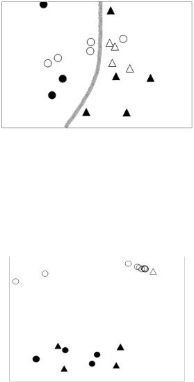
были поделены только на две группы: с низкой урожайностью (обозначаются треугольниками), и с высокой (обозначаются кружочками). Фигуры у объектов с отсутствующими измерениями тяжелых металлов не закрашены, а с имеющимися измерениями закрашены. На рисунке видно, что внутри каждого кластера имеется разделение на группы по урожайности. Причем в группе с измерениями тяжелых металлов это разделение более явное, поэтому можно предположить, что значения концентрации семи тяжелых металлов улучшают картину для анализа зависимости урожайности от комплекса показателей.

Теперь попробуем искусственно нивелировать неоднородность выборки, т.е заполнить отсутствующие измерения тяжелых металлов нами определенными значениями. Можно предположить несколько вариантов таких значений, например: минимальное из имеющихся измерений по конкретному металлу, максимальное, среднее и т.п., все они могут быть обоснованы только желанием проведения статистического эксперимента. Мы приведем результат, в котором пропущенные значения заменялись средними (рис. 2).

Рисунок 2. Модель для выборки 2019 г. по 17 показателям с «пустотами», замененными средними значениями

Этот результат ценен для нас тем, что кластеры, проявленные на рисунке 1, смешиваются так, что все равно можно провести (за исключением одного объекта) разграничение между расположением объектов по урожайности.

Перейдем к анализу выборки 2020 г. с посевами клевера 1 года пользования

(рис. 3).

Рисунок 3. Модель для выборки 2020 г. по 23 показателям с «пустотами».

408

Система обозначений сохраняется. Из рассмотрения были исключены параметры, по которым отсутствовали измерения, но объекты у которых имелись «пустоты», не исключались. Опять мы видим явное присутствие двух кластеров, в каждом из которых наблюдается структурирование. Для объектов с «пустотами» тот, который имеет наименьшую урожайность, занимает крайнюю позицию, а для объектов с полным набором данных есть как внешний контур с меньшей урожайностью, так и внутренний блок с высокой.

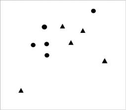
Для выборки 2021 г. ситуация с неоднородностью выборки остается. Мы приведем результат только для «урезанной» выборки, т.е. той, которая осталась после исключения показателей и объектов, где было хотя бы одно отсутствующее значение. Выборка таким образом сократилась до 10 объектов и 15 показателей. Это является вынужденным шагом, приводящим к сокращению объема статистического материала, который, наоборот, должен увеличиваться, потому что наши выводы по сути имеют асимптотический характер, т.е. доказываются при большом количестве объектов. И тем не менее, приведем данные полученной модели (рис. 4).

Рисунок 4. Модель для выборки 2021 г. по 15 показателям и 10 объектам

Большинство объектов структурируются в разделяемые кластеры, за исключением двух. К сожалению, не имеет смысла создать полноценную объединенную выборку за три года, поскольку каждая из них имеет свои проблемы. Объединенная выборка была бы меньше каждой из них по количеству точек и показателей, а мы должны проверять наши гипотезы на больших выборках.

Заключение. Отдельный анализ трех выборок позволяет нам сделать важные выводы:

•включение тяжелых металлов в комплекс показателей улучшает структурность моделей;

•метод многомерного шкалирования дает полезные результаты даже в условиях отсутствия значений некоторых показателей;

•даже на малых выборках прослеживается возможность разделения объектов, что может служить основанием использования предложенного

409

комплекса показателей для построения системы распознавания, построенной на современных нейросетевых алгоритмах.

Литература

1. Артюшкин В.Ф. Место БРИК в экономической и политической структуре мира (возможности применения метода визуализации многомерных структур) // Вестник МГИМО-Университета. 2010. № 1. С. 51-53.

2. Bortnik T. Yu., Artyushkin V.F. , Karpova A. Yu. Structural analysis of the productivity sample on a variety of factors characterizingsoil fertility (a possible approach to the solution)Earth// and Environmental Science, Volume 862, The VIII Congress of the Dokuchaev Soil Science Society 19-24 July 2021, Syktyvkar, Komi Republic, Russian Federation.

Environmental Science, Volume 862, The VIII Congress of the Dokuchaev Soil Science Society 19-24 July 2021, Syktyvkar, Komi Republic, Russian Federation.

УДК631.417.2; УДК 631.432.22

ХАРАКТЕРИСТИКА СВЯЗИ МЕЖДУ ВЛАЖНОСТЬЮ ПОЧВЫ И СТЕПЕНЬЮ ГУМИФИКАЦИИ ОРГАНИЧЕСКОГО ВЕЩЕСТВА С ИСПОЛЬЗОВАНИЕМ Q-MODEL

Д.Р. Бардашов1, А.Ю. Юрова2 1ФГБНУ ФИЦ Почвенный институт им. В.В. Докучаева, Москва, Россия

2Northwest Institute of Eco-Environment and Resources, State Key Laboratory of the Frozen Soil Engineering, Китай

e-mail: bardash@mail.ru

Аннотация. Исследованы взаимосвязи между степенью гумификации, легкостью минерализации почвенного органического вещества и влажностью почвы за счет сравнения эмпирических данных и результатов модельного эксперимента для черноземов Центрально-Черноземного заповедника.

410