

747 sensor network operation-1-187-3
.pdf16 SENSOR DEPLOYMENT, SELF-ORGANIZATION, AND LOCALIZATION
The PAMAS [10] multiaccess protocol saves power by switching off the radio of a node when it is not transmitting or receiving. This method saves power when idle listening consumes significantly less energy compared to message reception.
The Span approach [5] appears to be the most closely related to SCARE. Span attempts to save energy by switching off redundant nodes without losing the connectivity of the network. Nodes make decisions based on their local topology information. However, SCARE differs from Span in that it uses distance estimates to determine the state of a node. Span uses a communication mechanism to obtain this information. Since Span was developed for ad hoc networks, its main focus is on ensuring network connectivity through energyefficient topology management. It is not directed toward ensuring the sensing coverage of a given region. SCARE also differs from Span in that, in addition to ensuring network connectivity and low-energy self-configuration, it attempts to provide a high level of sensing coverage.
A TDMA-based self-organization scheme for sensor networks is presented in [11]. Each node uses a superframe, similar to a TDMA frame, to schedule different time slots for different neighbors. However, this scheme does not take advantage of the redundancy inherent in wireless sensor networks to power off some nodes.
SCARE utilizes a localization scheme for periodic transmission of beacon signals and for the synchronization of the clock signals of sensor nodes. A number of such localization schemes have been proposed in the literature for sensor networks [1–3]. These schemes use a special set of nodes, called the reference nodes, that transmit beacon signals to let the sensor nodes self-estimate their position. The approach in [12] is based on the received signal strength from the reference nodes to carry out location estimation of the sensor nodes. It is shown that despite fading and mobility, a small window average is sufficient to do location estimation.
Traditionally, GPS [13] receivers are used to estimate positions of the nodes in mobile ad hoc networks. However, their high cost and the need for more precise location estimates make them unsuitable for sensor networks. It is expensive to add GPS capability to each device in dense sensor networks.
In [14], a scheme is presented to estimate the relative location of nodes using only a few GPS-enabled nodes. It uses the received signal strength information (RSSI) as the ranging method. Whitehouse and Culler [15] use an ad hoc localization technique called Calamari in combination with a calibration scheme to calculate distance between two nodes using a fusion of radio-frequency (RF)-based RSSI and acoustic time of flight (TOF). Acoustic ranging [16] can also be used to get fine-grained position estimates of nodes.
Finally, several clustering techniques have been proposed in the ad hoc networking literature. Vaidya et al. [17] propose a scheme that attempts to find maximal cliques in the physical topology and use a three-pass algorithm to find the clusters. Although this scheme finds a connected set of clusters, it consumes a significant amount of energy during clustering and cannot be directly applied to sensor networks. The adaptive clustering scheme proposed in [18] uses node identifications (IDs) to build two-hop clusters in a deterministic manner. SCARE differs from this scheme in two ways. First, the main goal of SCARE is to use distance information to power down redundant sensor nodes, whereas in [18] node IDs are used to provide better QoS guarantees by clustering nodes. Second, in [18], as in [17], energy efficiency is a secondary concern. In [19], clustering schemes for both static and mobile networks are proposed. However, there is no provisioning for switching off redundant nodes in these schemes. Thus, [19] cannot be directly applied to sensor networks.

2.2 SCARE |
17 |
On the other hand, SCARE is specifically designed for sensor networks to take advantage of their inherent redundancy.
2.2.3 Outline of SCARE
SCARE is a decentralized algorithm that distributes all the nodes in the network into subsets of coordinator nodes and noncoordinator nodes. While the coordinator nodes stay awake and provide coverage and perform multihop routing in the network, noncoordinator nodes go to sleep. Noncoordinator nodes wake up periodically to check if they should become coordinators to replace failed coordinators.
SCARE achieves four desirable goals. First, it saves energy by selecting only a small number of nodes as coordinators and putting other nodes to sleep. Second, it uses only local topology information for coordinator election and hence is highly scalable. Third, it provides nearly as much sensing coverage compared to the coverage obtained if all the nodes are awake. Finally, it preserves network connectivity by using a protocol based on CHECK and CHECK REPLY messages. We next describe a basic scheme for self-configuration. The basic scheme will subsequently be extended to prevent network partitions.
Basic Scheme In self-configuration based on SCARE, each node starts by generating a random number with uniform probability between 0 and 1. A node becomes eligible to be a coordinator if the random number thus generated is greater than a threshold (say 0.9). Therefore, a very small percentage of the nodes actually become coordinators. Other nodes just wait and listen. The threshold value can be preset depending on the application. A higher value for the threshold results in a small number of initial coordinator nodes. This has the effect of delaying the convergence of the self-configuration algorithm, but it might result in a better selection of coordinator nodes. On the other hand, a low value for the threshold implies that a high number of coordinator nodes are selected randomly in the beginning. This hastens the convergence of the protocol although a larger number of coordinator nodes may be selected.
A node that is eligible to be a coordinator waits for a random amount of time before declaring itself to be a coordinator by broadcasting a HELLO message. This wait time, for example, can be chosen from a uniform distribution of values between T and N T where T is a preset slot time and N is the number of neighbors of the node that are coordinators. Initially N can be chosen to be a constant, for example, 6. This prevents excessive contention on the wireless channel that might result if all the nodes decide to become coordinators at once.
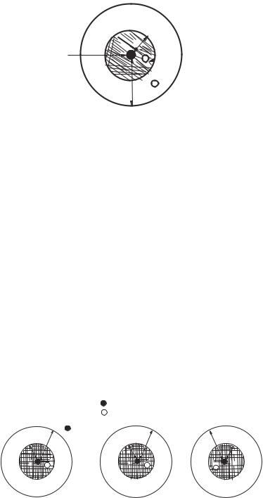
Upon receipt of a HELLO message, a sensor node compares its distance from the sender C of the HELLO message to its sensing range s. A node within a distance s from a coordinator immediately becomes a noncoordinator node and stores the ID of the node that sent the HELLO message in its local cache. A node that is at a distance greater than s from C but within transmission range r becomes eligible to be a coordinator node. This is shown in the Figure 2.1. The shaded region in the figure represents the sensing range of the node C. The outer circle represents the transmission range of the sensor node. Here, we assume that the sensing radius is smaller than the transmission radius. This is often the case for sensors in a sensor node [20].
While SCARE assumes the presence of an appropriate localization mechanism [1–3], exact distance calculations are not necessary. We show later that a moderate error in distance estimation has little effect on the outcome of the self-configuration procedure.
18 SENSOR DEPLOYMENT, SELF-ORGANIZATION, AND LOCALIZATION
r = transmission radius |
s = sensing radius |
C s
Coordinator
r
Eligible to be  noncoordinator
 Eligible to be coordinator
Figure 2.1 Sensing and transmission radii of a node.
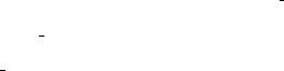
Network Partitioning Problem The basic scheme described above can sometimes result in a partitioning of the network; see Fig. 2.2a. Here, coordinator node F makes node A a non-coordinator. However, coordinator node D can communicate with F only through A. This can potentially result in the partitioning of the network if coordinator (active) node D is unable to reach any other active nodes. As a result, network connectivity cannot be guaranteed in this situation. In Figure 2.2b, G and K are coordinator nodes and B and C are noncoordinator nodes. This situation again results in network partitioning as nodes G and K cannot reach each other.
To prevent such situations, we extend the basic SCARE scheme outlined above, which results in a more effective technique for self-configuration. In the basic scheme, if there is a network partition, a node might never receive a HELLO message. This results in the node waiting eternally for a HELLO message, which results in wastage of energy. Hence, we choose a time-out value Toff after which the nodes that are still undecided about their state can become eligible to become coordinator nodes. The time-out value can be chosen based on the probability threshold discussed in Section 2.2.3. A lower value for the threshold means that the procedure converges quickly and needs a lower Toff value and vice versa.
To prevent the network partitioning that occurs due to the pathological cases shown in Figure 2.2, a node that initially receives a HELLO message from a coordinator node does not become a noncoordinator immediately and go to the sleep state. Instead, it continues to listen for messages from other coordinator nodes and remains in the “eligible to be a
|
|
|
Coordinator |
s = sensing radius |
||
|
|
|
Noncoordinator |
r = transmission radius |
||
|
r |
|
D |
r |
r |
|
|
|
|
|
|||
|
|
|
|
|
||
s |
|
A |
s |
B |
C |
s |
F |
|
G |
K |
|||
|
|
|||||
|
|
|
|
|||
(a) (b)
Figure 2.2 Network partitions in the basic scheme: (a) first scenario and (b) second scenario.
2.2 SCARE |
19 |
noncoordinator” (ETNC) state. A sensor node that is in the ETNC state can become a coordinator node in two cases:
1.If it can connect two neighboring coordinator nodes1 that cannot reach each other in one or two hops. It can deduce this information from the HELLO messages it received earlier. As shown in Figure 2.2a, node A, which is in the ETNC state, receives HELLO messages from node F and node D and decides to become a coordinator; this eliminates the partition.
2.If it can connect two neighboring coordinator nodes that cannot reach each other in one or two hops via a node in the ETNC state. As shown in Figure 2.2b, nodes B and C, that are in the ETNC state, receive HELLO messages from nodes G and K, respectively, and decide to become coordinators as there is no match between the node lists of G and K; this eliminates the partition.
To achieve this, each ETNC node sends a CHECK message. This CHECK message contains the neighbor list of the coordinator node that caused this node to be in the ETNC state. Intuitively, this case is more likely to occur if there are few coordinators in the vicinity and less likely if there are more coordinator neighbors. Any ETNC node that receives this CHECK message replies with a CHECK REPLY message and becomes a coordinator if there is no node common to the neighbor lists of both the nodes. Upon receipt of the CHECK REPLY message, the node that sent the CHECK message also becomes a coordinator. In Figure 2.2b, noncoordinator node B sends a CHECK message and gets a CHECK REPLY message from node C. Both nodes B and C, therefore, become coordinator nodes. This procedure removes the network partition.
If the HELLO message is received from the same partition, and the node lists contained in the HELLO message do not have any common neighbors with the node lists the node received from other HELLO messages, then the node goes from the ETNC state to the “eligible to be coordinator” (ETC) state. This removes partitions if the HELLO messages are from different partitions. If they are from the same partitions, then the node connects the two coordinator nodes.
To prevent oscillations during the selection of coordinators, we enforce the condition that once a node becomes a coordinator, it continues to remain a coordinator until it is unable to provide any service. This strategy is used despite the fact that this coordinator might become redundant later during self-configuration. This penalty is reasonable since it occurs infrequently, especially in contrast to the energy needed to select an optimum number of coordinators. As the density of nodes increases, the fraction of noncoordinator nodes increases, and this leads to more energy savings. Due to its distributed nature, SCARE has a slightly larger number of coordinators than the minimum number necessary for coverage and connectivity. This also happens due to the randomness involved in the distributed selection of coordinator nodes.
After self-configuration, each coordinator periodically broadcasts a HELLO message along with a list of its one-hop neighbors that are coordinators. Noncoordinator nodes listen to these messages. Noncoordinator nodes also maintain a timer to keep track of the coordinator node that made them a noncoordinator. If this timer goes off, a noncoordinator
1 A neighboring node lies within the node’s transmission radius.