книги / Разработка нефтяных и газовых месторождений. Ч. 2

Testing methods considering additional fluid influx. Non-instantaneous influx stop greatly distorts pressure build-up curves. In the long run, pressure build-up curve asymptotically tends toward curve that corresponds to instantaneous bottomhole zone closing. However, it is connected with long-term well shutdown, especially stripper well, and it is often unacceptable for production well operation.

To reduce the testing time, the special methods for processing pressure buildup curve considering influx have been created. There are several methods for processing pressure build-up curve considering influx processing. Let us discuss the method which the most widely used in Perm Krai – ShchelkachevKundin method.

Cumulative fluid influx or amount of fluid flowed from formation to well at any time t after well shutdown (fig. 9) can be determined by formula:

ρ is fluid density under reservoir conditions; and

∆pзаб, ∆pзатр, ∆pбуф are, respectively, bottomhole pressure, annulus pressure and flowing tubing head pressure.

Fig. 9. Well 212, Vysokovskoye Field. Flow Rate Curve

61

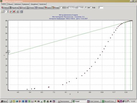
Thus, if at the end time point of pressure build-up measurement t inflow is still going on, it is necessary to process the pressure build-up curve considering influx. By quadratic approximating the continuing fluid influx on the basis of superposition method, we obtain the below expression:

where Q(t/2) is continuing fluid influx that corresponds to time t/2 from well shutdown time.

The above expression is a straight line equation (fig. 10):

Angle of inclination can be determined in a way similar to determination by tangent method, and hydroconductivity is determined by formula:

Fig. 10. Well 212, Vysokovskoye Field. Pressure Build-up Curve,

Shchelkachev-Kundin Method

62

1.3. PRESSURE INTERFERENCE TEST

Pressure interference test is surveillance of well pressure change caused by changing fluid withdrawal or fluid injection in the neighboring wells of the same reservoir or neighboring reservoirs.

For pressure interference testing, two wells should be selected. One well acts as disturbing well (shutdown and return) and the second well is responsive well. Both wells must be hydrodynamically studied for preliminary calculation of expected pressure surge arrival time from the disturbing well to the responsive well.

In the course of testing, for at least 2 pressure surges at definite frequency should be made (fig. 11). Meanwhile, all wells with the test area shall not change operation conditions for reducing noise.

Fig. 11. Well 337, Unievinskoye Field. Formation Pressure Change under Pressure Interference Test

Pressure interference test methods can be characterized by high resolution, and, in addition to hydroconductivity, they make it possible to determine expressly reservoir piezoconductivity – parameter that characterizes elastic properties of reservoir and reservoir fluid, and bonding strength. If integrated with other

63

methods, such test makes it possible to obtain data of reservoir homogeneity and identify lithological screens.

2. PUMPING WELL PERFORMANCE APPRAISAL HYDRODYNAMIC STUDY PACKAGE

2.1. RESERVOIR DELIVERABILITY APPRAISAL

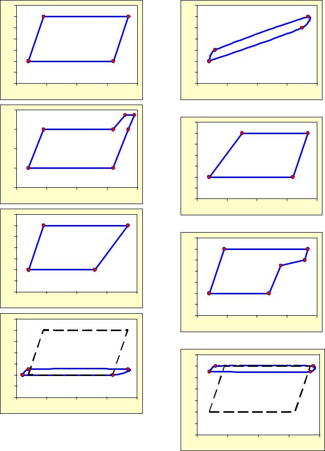
Pumping wells are the major part of the OOO LUKOIL-PERM production well stock. In flowing well, pressure at any depth can be directly measured by lowering pressure gage, but such procedure is impossible in pumping well – bottomhole pressure is determined by indirect data – it is necessary to determine fluid level in annulus space using acoustic level meter (fig. 12). The level meter is comprised of acoustic signal generation device and acoustic signal receiving device, which includes microphone, pressure sensor and analog signal digitizer. Measured data – level depth, annulus pressure, acoustic sound velocity, acoustic wave transmission dataset (echogram – fig. 13) is automatically recorded in nonvolatile memory of recording unit connected to the level meter with cable. Reference data – well number, well cluster number, operator code and test date are entered manually and saved in the nonvolatile memory of the recording unit. The level is determined by known relationship between distance to the level and acoustic signal transmission time:

Acoustic sound velocity is determined by pressure correction tables because it is known that acoustic sound velocity depends on fluid pressure. Such pressure correction tables are available for each OOO LUKOIL-PERM field. They are stored in nonvolatile memory of recoding units and are available for each test operator. If we know level and curvature, fluid column and bottomhole pressure at any point of borehole can be calculated by formula:

where Нпр is depth datum for determining Рзаб, m;

ρжид is fluid density in well, kg/m3; and

Рзатр is wellhead annulus pressure, MPa.

64

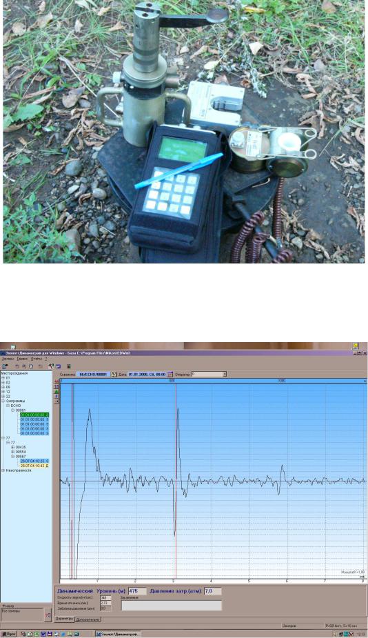
Fig. 12. MIKON-101 Digital System, Level Gage, DN-117 Attached

Dynamometer, DV-118 In-Built Dynamometer

Fig. 13. Echogram

65

Such method is used for determining steady-state flow and unsteady-state flow pressure. Since each pump is fitted with check valve, fluid flows to annulus space under fluid level increase and wellhead pressure increase. By recording level change within the time period before changing stops, we obtain pressure build-up curve that is plotted in coordinates ∆p (rc, t), ln(T+t)/t or ∆p (rc, t), ln t. Then, reservoir deliverability should be determined using the above described methods.

2.2. SUCKER ROD PUMPING

WELL PERFORMANCE APPRAISAL

If development targets occur not deep (depth of occurrence is up to 1500 m), the major part of pumping well stock is sucker rod pumping wells. Sucker rod pumps are brought into operation by conventional pumping units installed at wellhead. Sucker rod pump performance is determined by dynamometry: dynamometer measures loads on sucker rods under subsurface pumping unit operation.

Measurements are taken near the sucker rod hanger centers – at the top end of polished rod. There are overlay (attached) dynamometers and dynamometers with equalizer beam sensors (fig. 2.1.1). In the first case, dynamometer sensor is installed directly on the polished rod (near sucker rod hanger center), and in the second case, it is installed in the equalizer beam space (equalizer beam is point of hanger and polished rod joint). Attached dynamometer operating principle is direct measuring polished rod diameter and calculating load that causes polished rod diameter change (by lateral and longitudinal deformation). Equalizer beam dynamometer operating principle is direct measuring polished rod load change by strain-gauging and polished rock moving. All signals are digitized for dynamometer chart building-up and processing.

Under normal operation of subsurface pumping unit, sucker rods are exposed to tensile stress (Р), but such stresses are different at different time. Let us discuss such stresses and nature of the stresses using dynamometer chart (fig. 14), where

Sшт is polished rod stroke length, and Р is sucker rod load. Segment АБ corresponds to initial period of polished rod upstroke – tensile stress becomes higher. Point Б corresponds to the time of standing valve opening. In interval БВ sucker rod upstroke is still going on if sucker rod load is constant and equal to

Р2. In interval ВГ sucker rod downstroke begins – fluid column weight is

66

removed from sucker rods. In point Г traveling valve is opened. In interval ГА

(sucker rod downstroke is still going on) load is minimal and is equal to Р1. The distance бВ=Sшт characterizes the polished rod stroke; the distance БВ = Sпл corresponds to plunger stroke, and segment бБ – deformation of sucker rods and pipes.

Fig. 14. Theoretical Dynamometer Chart

The most typical dynamometer charts are given in fig. 15:

a)actual dynamometer chart;

b)plunger sticking – the entire stroke is used for sucker rod stretching out, and it is reduced while downstroke;

c)plunger seizure at the end of upstroke;

d)fluid leaks through traveling valve and plunger and pump barrel clearance increases during plunger upstroke;

e)fluid leaks through standing valve during plunger downstroke;

f)free gas in pump;

g)complete failure of traveling valve; and

h)complete failure of standing valve.

67

2.3. HYDRODYNAMIC STUDY SOFTWARES AND TECHNIQUES

At present, high-precision digital instruments (MIKON, SKAT and other) manufactured in Russia and France (PPS) are used for all hydrodynamic studies performed in the OOO LUKOIL-PERM fields. The leading role in performing researches within the territory of Perm Krai belongs to OOO Universal-Service. All hydrodynamic study data are processed by special software products PanSystem and IRIS. IRIS was specially developed by PermNIPIneft institute.

Application of software products makes it possible to determine oil reservoir deliverability, reservoir fluid flow patterns, reservoir model, boundaries and type. Of high importance are methods used for obtaining pumping well data on a real-time basis, and it makes it possible to exercise on-line control over well operation and reservoir development systems. Such methods include well operation data obtaining by instruments installed under subsurface pump for the entire turnaround. They are widely used within OOO LUKOIL-PERM, and OOO Universal-Service developed a special technique for running fixed apparatus under subsurface pump.

According to that technique, bottomhole apparatus is installed in special holder under subsurface pump which is connected by logging cable and data are obtained on a real-time basis (fig. 16). Such bottomhole apparatus records data automatically in nonvolatile memory. Operator’s duty is just to take regular readings from nonvolatile memory and transmit them by electronic communication channels. Such technique does not require any modifications and changes in wellhead equipment, the bottomhole apparatus is run simultaneously with pump running.

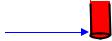
9 10

Fig. 16. Bottomhole Apparatus Layout under Borehole Pump

69

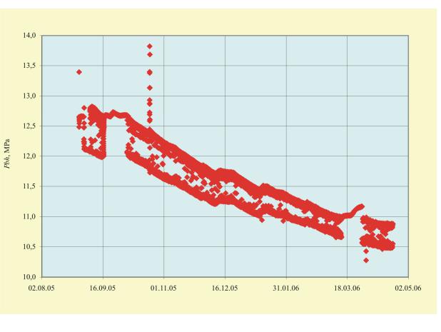
Such technique has been used in the OOO LUKOIL-PERM fields since 2004. Today, more than 50 wells in 13 fields are equipped with such bottomhole apparatus which provide data on a constant basis. For illustration, data for well 212, Shershnevskoye field (Yasnopolyanskaya reservoir) (fig. 17) is provided. The above well is operated in periodic mode (extraction + accumulation), and relationship between reservoir energy change and reservoir development operations can be clearly seen due to applying the above technique.

Our experience in such technique application shows that obtained data make it possible:

•to obtain reliable bottomhole pressure data on a real-time basis;

•to monitor energy state of not only well but also large part of reservoir for the long-term well operation;

•to exercise on-line control over enhanced oil recovery efficiency in development target; and

•to perform well hydrodynamic studies, including pressure interference test without any production loss.

Fig. 17. Well 212, Shershnevskoye Field. 12/12 Operation.

Pump Intake Pressure

70