Учебное пособие 2161

Russian Journal of Building Construction and Architecture

rating environment (not shown in Fig. 1). The centering flange 11 is joined with the collector of the operating environment (not shown in Fig. 1). The shaft 7 on the external side of the hollow body 1 is joined with the rotation source (not shown in Fig. 1) which should be able to change its own rotation frequency for that of the generation of the impulses of the amount of movement to be controlled. E. g., this can be an electric engine with the rotation frequency of the shaft controlled by a frequency transformer.

The shaft 7 is rotated in such a manner in relation to the centering flange 11 put into the first extra inlet 13 of the hollow body 1 and the directing bushing 12 installed in the second extra inlet 14 of the hollow body 1. As a result, the cam 8 connected with the shaft 7 starts rotating. As the cam 8, which is an involute curve, rotates, alternating reciprocating movement of the first rod 5 in the first bushing 6 and the second rod 18 in the second bushing 19 is provided. As the first shock valve 4 is rigidly fixed on the first rod 5 and the second shock valve 17 is rigidly fixed on the second rod 18, during the alternating reciprocating movement of the rods 5, 18 there is opening and closure of the end-to-end ducts 15, 20 alternately in the first 6 and the second 19 bushings.

The cam 8 contributes to the opening of the first and second shock valves 4, 17 as the shaft 7 rotates in the first and second rods 5, 18. The first spring 9 which is installed in the first rod 5 using the first retaining ring 10 contributes to the stretching closure of the first shock valve 4. The second spring 21 which is installed in the second rod 18 using the second retaining ring 22 contributes to the closure of the second shock valve 17.

Then the operating environment is supplied through the hollow body 1 from its source to the collector. As a result, the operating environment finds its way into the hollow body 1 through the end-to-end ducts 15 of the first bushing 6 and/or the end-to-end ducts 20 of the second bushing 19 and leaves it through the end-to-end cuts 16 in the centering flange 11. As the rotation of the cam 8 of the shaft 7 provides alternating opening of the end-to-end ducts in the first 6 and second 19 bushings, there is a hydraulic shock (from the inlet of the operating environment) as the inlet section of the first bushing 6 is completely closed with the first shock valve 4. At this moment the operating environment is accelerated using the second bushing 19. As the inlet section of the second bushing 19 is completely closed with the second shock valve 17 (from the inlet of the operating environment), a hydraulic shock is also generated and at this moment the operating environment is accelerated through the first bushing 6.

Changes in the rotation frequency of the shaft 7 provide those of the frequency of the alternating generation of hydraulic shocks of the operating environment in the first 6 and second 19 bushings independently of its consumption through the end-to-end cuts 16 of the centering flange 11.

20

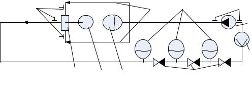
2. Developing an experimental setup for investigating the characteristics of a shock node of an opposite structure with external operation of the valves. A scheme of an experimental setup for investigating the above structure of a shock node is presented in Fig. 2.

Fig. 2. Scheme of the experimental setup: 1 is a pump; 2 is an electromagnetic transformer of the consumption; 3 are reverse valves of a rectifying system of the consumption of the operating environment;

4 is a hydraulic accumulator at the inlet of the shock node; 5 is a gear motor; 6 is a shock node with possible external operation; 7 are pressure transformers for investigating the operation of the shock node;

8 are alimetary pipes; 9 are rectifying hydraulic accumulators of the rectifying system of the consumption of the operating environment; 10 – +pressure transformers for controlling the operating parameters of the pump

This scheme solution operates in the following way. The pump 1 feeds the operating environment along the closed hydraulic contour alternately through the alimentary pipes 8 switched to the inlets of the shock node 6 (see Fig. 1). At the outlet of the shock node 6 the operating environment is fed into the sequential hydraulic accumulators 9 of the rectifying system of the operating environment through the reverse valves 3. Then it is again fed into the pump inlet 1 through the electromagnetic transformer of the consumption 2. The extra hydraulic accumulator 4 installed at the joint of the alimentary pipes 8 at the inlet of the shock node 6 serves to protect the pump 1 from distribution of the hydraulic shock and is also a stabilizer of the shock node 6 of the opposite structure.

Pressure pulsation in the alimentary pipes 8 as well as at the outlet of the shock node 6 is measured using the pressure transformers 7. The pressure at the inlet and outlet of the pump 1 is controlled using two pressure transformers 10.

The consumption of the operating environment is measured using the consumption transformer 2 at the outlet of the hydraulic accumulators 9 of the rectifying system of the consumption. Changes in the frequency of the opening of the shock valves of the shock node occur by means of those in the frequency of the rotation of the gear motor 5.

The shock node (Fig. 3) is made of cross bar G3/4 and two reverse valves G3/4 in accordance with the patented technical solution described above. A hydraulic contour is assembled

21

Russian Journal of Building Construction and Architecture

from metal pipes with the diameter 50 mm and polypropylene PP-R pipes with the diameter 25 mm using standard piping fittings G1/2 , G3/4 , G1 , G3/2 and G2 (Fig. 3). The length of the shoulders of the alimentary PP-R pipes at the inlet of the shock node (Fig. 2) to their joining point is 1.3 m.

The consumption of the operating environment in the closed hydraulic contour was provided with a pump “К 80––50––200A” with an asynchronous engine “АИР 132М2Y2” with the power 11 kWatt. Changes in the productivity of the pump were made using the frequency transformer “ОВЕН ПЧВ-2”.

The handle of the shock node of the opposing type with external operation of the opening moment of the shock valves was operated using an electric engine “AIS 71C4” with the power 0.55 kWatt through a reducing reductor “NMRV040”. Changes in the rotation frequency of the electric engine and thus that of the opening of the valves of the shock nodes were made by means of a frequency transformer “MINI––L––4T0007M”.

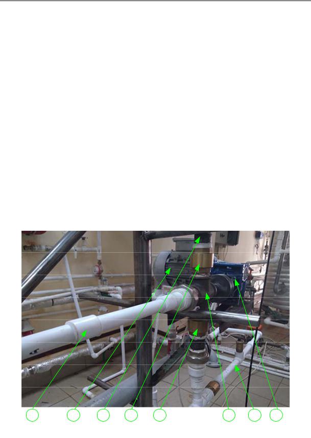
A fragment of the experimental setup containing a shock node of the opposite structure with possible external operation of its valves switched to the gear motor is given in Fig. 3.

Fig. 3. View of the experimental setup: 1 is a pipe of the outlet of the operating environment from the shock node; 2 is an electric engine; 3 is the first alimentary pipe for the oepration of the shock node;

4 is the first shock valve; 5 is the second shock valve; 6 is the body (cross bar G3/2 ) of the shock node; 7 is the second alimentary pipe for the operation of the shock node; 8 is a reducing reductor

22

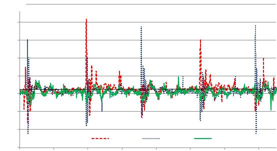
3. Results of the experimental studies. The results of the experimental studies of the shock node are presented in Fig. 4––6. Fig. 4 presents a graph of pressure pulsations generated by the shock node with the frequency 1.5 Hz at the consumption of the environment 0.1763 m3/h with available head pressure at the inlet 50 kPа.

Fig. 4. Pressure pulsations occurring during the operation of the shock node of the opposing type with external operation of its valves: 1 is the first inlet of the operating environment; 2 is the second inlet of the operating environment; 3 is the outlet of the operating environment from the shock node

Fig. 4 suggests that at the specified perimeters a pressure increase at the moment of a hydraulic shock reaches (530 ±30) kPа. The observed divergence in the pressure growth at the inlets of the shock node during periodic hydraulic nodes is due to a short length of alimentary pipes (1.3 m) and a small volume of the hydraulic accumulator installed at their joining point (see Fig. 2) that are not capable of ideal repetition of initial conditions for generating the impulses of the amount of movement of the operating environment for this particular consumption. However, unlike the self-powered structure [4], this has no effect whatsoever on the stability of the operated shock node as it retains a stable frequency of the generation of the impulses of the amount of the movement in the operating environment. The above graph suggests that the impulse mode of the circulation of the operating environment is observed only at the inlets of the shock node, i. e. a sharp increase in the pressure is accompanied by its sharp decrease as the conditions for cavitation of the operating environment are created. At the outlet of the shock node of the opposite type the character of changes of the operating environment which

23

Russian Journal of Building Construction and Architecture

is pulsing almost like a sine curve, i. e. the pressure growth of the operating environment is identical to the pressure decrease. The graph in Fig. 4 is also a basis for the dependences of a pressure increase during the hydraulic shock on changes in the consumption of the operating environment and changes in the frequency of valve switching (Fig. 5 and 6).

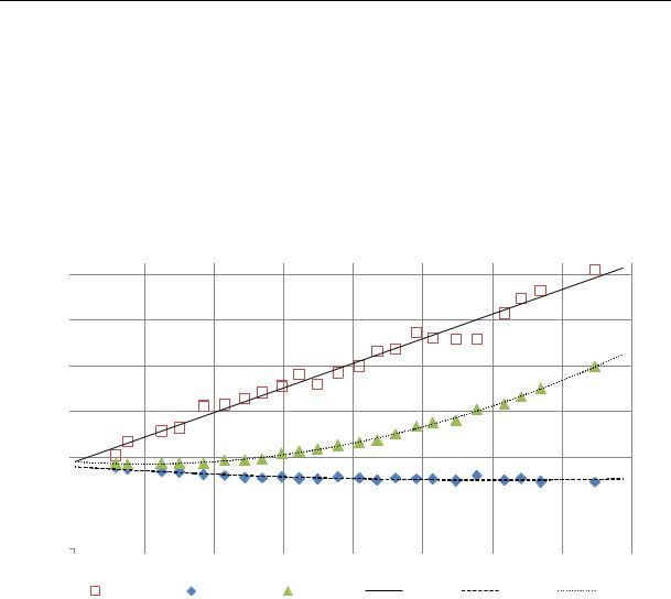
The dependence of changes in the pressure growth of the operating environment at the moment of the hydraulic shock on changes in the consumption of the operating environment through the setup at the constant frequency of valve switching of 1.5 Hz is in Fig. 5.

Fig. 5. Changes in the pressure at the characteristic points of the closed hydraulic contour in relation to the atmospheric pressure during those in the consumption of the operating environment:

1 is the pressure growth at the moment of the hydraulic shock at the inlet of the shock node (experimental data); 2 is the pressure at the inlet of the pump (experimental data); 3 is the pressure at the outlet of the pump (experimental data); 4 is Excel approximation for the dataset 1; 5 is Excel approximation for the dataset 2;

6 is Excel approximation for the dataset 3

Fig. 6 presents the results of a study of dependence of pressure change at characteristic points of a closed hydraulic contour in relation to the atmospheric pressure when available head pressure of the contour is maintained at 130 kPа and changes in the frequency of the valves of the shock node range from 0.1 to 2.5 Hz.

Fig. 5 suggests that the pressure growth at the moment of the hydraulic shock has a linear character depending on changes in the consumption of the operating environment. The resulting approximation equation characterizing the dependence is highly agreeable with the results of theoretical studies by V. M. Ovsepyan in [6, p. 25].

24

900

P, kPа

800

700

R² = 0.8545

600

500

400

300

200

100

Fig. 6. Pressure changes at the characteristic points of a closed hydraulic contour in relation to the atmospheric pressure when available head pressure is maintained at 130 kPа when the frequencies of valve switching of the shock node change: 1 is the maximum pressure growth at the moment of the hydraulic shock (experimental data); 2 is the averaged pressure at the inlet of the pump;

3 is the averaged pressure at the outlet of the pump; 4 is Excel approximation for the dataset 1

Fig. 6 suggests that the pressure growth at the moment of the hydraulic shock has a distinct maximum at the frequency of around 1.5 Hz. This is due to the fact that at a smaller frequency of valve switching, which characterizes their smoothness an incomplete hydraulic shock. At a higher frequency of valve switching the consumption of the operating environment through the shock node is not able to reach its maximum corresponding with the available head pressure of 130 kPа and resistance of the hydraulic system.

4. Mathematical modeling of the shock node. Reliable and efficient reaction of a shock node during generation of periodic hydraulic shocks in a certain setup is characterized by the closing time of the valve t, seс which should be less than some design value tp, seс when a hydraulic shock wave reaches the distance equaling two alimentary pipe lengths. The valve should close before a reflected hydraulic shock wave reaches it when it is open, i. e. the following equation should hold

where t is the current closing time of the valve, seс; tp is the design closing time of the valve, seс; L is the length of an alimentary pipe, m; a is the distribution rate of the hydraulic shock wave, m/seс.

25

Russian Journal of Building Construction and Architecture

The current closing time t, seс of the valve of the hydraulic shock should be given by changes in the rate v, m/seс using the ratio

Change in the rate v, m/seс, can be predicted using the amplitude and frequency characteristics obtained using the force and rate growth. These characteristics are easy to design energy chains are used.

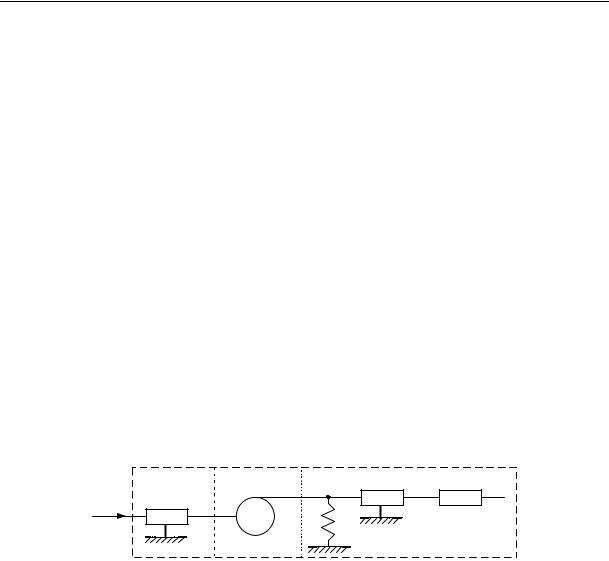
The energy chain of the shock node when the valve closes has 3 links (Fig. 7): the first one is hydraulic which accounts for the hydraulic resistance of the valve using the active resistance r1, (kPа·seс2)/l2; the second one is transformative, it transforms the pressure Р1, kPа, and the volumetric consumption V, l/sec, into the force f, H, and the linear rate v, m/sec, respectively; the third link is mechanical, it accounts for the properties of the spring-loaded valve with the deformation l, m/Н, mechanical friction for active resistance friction r2, (Н·seс)/m, and inertia properties with the mass т, kg, of moving parts of the valve.

1 2 3

Fig. 7. Energy chain of the shock node when the valve closes: P is the pressure of the operating environment at the inlet of the shock valve, kPa; V is the volumetric consumption of the operating environment through the shock node, l/sec; r1 is the hydraulic (active) resistance of the valve, (kPа·seс2)/l2; Р1 is the pressure of the operating environment at the outlet of the valve considering the hydraulic (active) resistance of the valve, kPа; f is the force on the valve from the inlet of the operating environment, H; v is the linear closing rate of the valve, m/seс; l is the deformation of the spring-loaded valve, m/Н; v1 is the linear closing rate of the valve considering a

drop in the rate of its deformation, m/seс; r2 is the mechanical (active) resistance of the valve, (Н·seс)/m; f1 is the force of the valve from the inlet of the operating environment, H; m is the mass of the valve and other moving parts of the shock node, kg; f2 is the force on the valve from the inlet of the operating environment, H;

S is the section area of the valve, mm2

26

Let us present the outlet parameters of the chain as the sum of the constant component and deviation:

Using the substitute

27

Russian Journal of Building Construction and Architecture

The basic parameters for the scheme of the experimental setup are as follows: r1 = 50 (kPа seс2)/l2; r2 = 1 (Н seс)/m; l = 0.075 m/Н; т = 0.15 kg; S = 490.625 mm2 (at the valve diameter d = 25 mm); V20 = 0.2 l/seс.

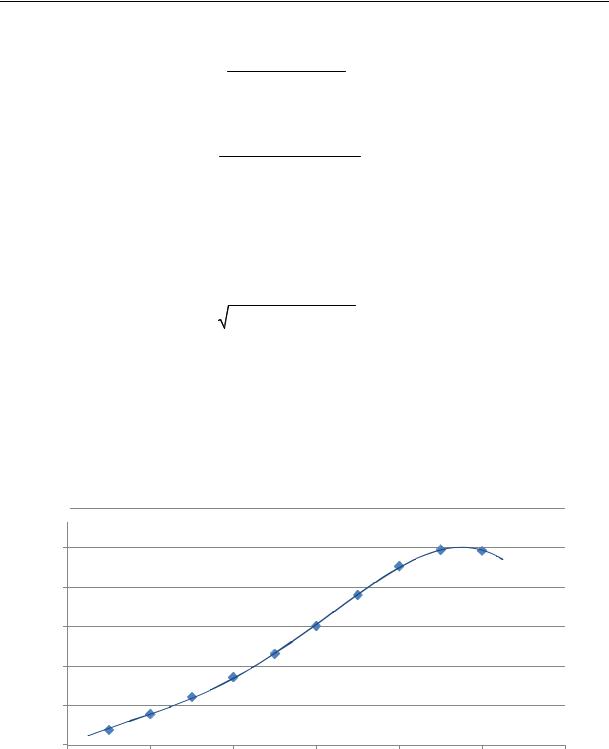
Based on the expressions (17)––(19) the graph of the amplitude and frequency characteristics will be as presented in Fig. 8.

A1,2(jΩ)

1

R² = 0.9997

0,8

0,6

0,4

0,2

0

Fig. 8. Amplitude and frequency characteristics of the energy chain when the valve closes with the basic parameters of the energy chain

Fig. 8 suggests that the amplitude and frequency characteristics A(jΩ) reaches its maximum at the angular rate Ω ≈ 9.4 rad/seс, which corresponds with the cam frequency f = 1.49 Hz and rate change v = 1 m/seс. Considering the actual gap between the valve and its seat δ = 5 mm,

28

based on the formula (2) the current closing time of the valve at the moment is t 0.0051 0.005sek.

The design time for reaching the effective operation of the hydroshock node at the alimentary pipe length L = 1.3 m and the distribution rate of the hydraulic shock in a PP-R pipe а = 398 m/seс given by the formula by N. Ye. Zhukovskiy [6, p. 105] based on the formula

(1) we get

tр 2 1.3 0.0065 sek. 398

Since at the angular speed Ω ≈ 9,4 rad/seс the time is t > tp, the shock node will operate effectively according to the mathematical modeling condition (1).

The sufficiency of the mathematical modeling is proved by the results of experimental studies presented in Fig. 6 where the maximum pressure increases at the moment of the hydraulic shock was also observed at the valve switching frequency of around f = 1.5 Hz. Considering that, Fig. 9––12 present the results of mathematical modeling of the shock node when the valve closes with a variation in the most significant parameters of the energy chain according to the Table.

Fig. 9 suggests that as the mass of the moving parts of the shock node increases, the maximum possible rate change at the moment of the hydraulic shock v, m/seс, decreases and so

29